In This Article
- 1. Origins of the Monte Carlo Method
- 2. Why Monte Carlo in Medical Physics?
- 3. Monte Carlo Codes: EGS, MCNP and GEANT
- 4. The EGS Code System: From Shielding to Dosimetry
- 5. Electron Transport and Condensed History
- 6. Ion Chamber Dosimetry
- 7. Early Radiotherapy Applications
- 8. Monte Carlo vs. Deterministic Methods
- 9. The Future of Monte Carlo
Origins of the Monte Carlo Method

The Monte Carlo method provides numerical solutions to problems described as the temporal evolution of objects — in medical physics, quantum particles such as photons, electrons, neutrons and protons — interacting with other objects based on cross-section relationships. Rather than solving transport equations analytically, the method directly simulates a system’s microscopic dynamics, randomly processing interaction rules until numerical results converge to reliable estimates of means, moments and their variances. In principle, Monte Carlo is simple: it solves macroscopic systems by simulating microscopic interactions. The geometry of the environment, so critical in deterministic approaches, plays only a secondary role — it defines the local environment of objects interacting at a given place and time.
Series overview: for the full roadmap and related articles, return to the complete guide on Monte Carlo in radiotherapy.
Stochastic sampling methods existed well before computers. In 1777, Comte de Buffon proposed a Monte Carlo-like experiment: repeatedly tossing a needle onto a ruled sheet of paper to determine the probability of the needle crossing one of the lines. For a needle of length $L$ tossed on a plane ruled with parallel lines spaced a distance $d$ apart (where $d > L$), the crossing probability is given by:
$$p = \frac{2L}{\pi d}$$
Where:
- $p$ = probability of the needle crossing a line
- $L$ = needle length
- $d$ = distance between parallel lines ($d > L$)
Laplace later suggested this procedure could determine the value of $\pi$, albeit slowly. The modern era began with Stan Ulam, who, while convalescing from an illness, played solitaire repeatedly and wondered whether he could calculate the probability of a successful play by combinatorial analysis — or simply by playing a large number of games and tallying results. In his autobiography, Ulam wrote: “The idea for what was later called the Monte Carlo method occurred to me when I was playing solitaire during my illness.”
Ulam shared this insight with John von Neumann, who was then working alongside Metropolis on theoretical calculations for thermonuclear weapons at Los Alamos. Precise neutron transport calculations are essential in designing thermonuclear weapons — the atomic bomb trigger destroys instrumentation before useful signals can be extracted, so simulation was the only viable approach. Von Neumann was especially intrigued. The first documented suggestion of using stochastic sampling methods for radiation transport appeared in correspondence between von Neumann and Richtmyer on March 11, 1947, proposing the use of the ENIAC computer. Shortly after, Metropolis and Ulam published their founding paper, “The Monte Carlo Method” (1949) — the first unclassified work to associate the name “Monte Carlo” with stochastic sampling.
Already by 1949, symposia were organized focusing on Monte Carlo applications in mathematical techniques, nuclear physics, quantum mechanics and general statistical analysis. The 1954 Symposium on Monte Carlo Methods at the University of Florida proved especially important: 70 attendees, many recognized as “founding fathers” by Monte Carlo practitioners, presented 20 papers spanning 282 pages plus a 95-page bibliography. A remarkable irony underlies this history: a mathematical method created for the most terrible weapon in history — the thermonuclear bomb, which has never been used in conflict — ended up benefiting millions through its medical applications.
Why Monte Carlo in Medical Physics?
Monte Carlo is often viewed as a “competitor” to deterministic and analytical methods. In practice, a scientist should always ask: what do I want to accomplish, and what is the most efficient path? The most successful researcher will use more than one method of approach.
Two fundamental realities exist. First, macroscopic transport theory provides deep insight and builds sophisticated intuition about how particle fields behave — Monte Carlo cannot compete well here. Monte Carlo practitioners work much like experimentalists, discovering properties of macroscopic field behavior through trial and error, guided by intuition. Second, when complexity grows, Monte Carlo simulations become the most advantageous method. A mathematical proof in the book’s appendix demonstrates that Monte Carlo is more efficient than deterministic approaches once the problem dimensionality exceeds four — and radiotherapy problems typically occupy dimension 6 or 7.
The rise of linear electron accelerators (LINACs) in radiotherapy directly drove the need for Monte Carlo dose prediction and dosimetry. LINACs produce energetic, penetrating photon beams that enter deep into tissue, sparing the surface and attenuating considerably less rapidly than $^{60}\text{Co}$ or $^{137}\text{Cs}$ beams. Relativistic electrons have a range of approximately 1 cm per 2 MeV of kinetic energy in water, and the diameter of the electron energy deposition “plume” — pear-shaped at its maximum — is also about 1 cm per 2 MeV. These dimensions match the organs being treated and organs at risk. Treatment areas are heterogeneous, with differences in composition and density, and the instruments used to measure dose are even more diverse. It remains true today that Monte Carlo provides the only prediction of radiometric quantities satisfying the accuracy demands of radiotherapy.
The scale of Monte Carlo research underscores its importance: as of 2020, about 900,000 papers had been published on Monte Carlo methods, with nearly 55,000 related to medicine — a consistent 10%–20% contribution since at least 1970. Before 2005, growth appeared exponential in both areas. Since then, the medical curve leveled out at over 3,000 publications per year.
Monte Carlo Codes: EGS, MCNP and GEANT
Three code systems have historically dominated Monte Carlo simulations in medical physics and radiotherapy. Each has distinct origins, strengths and communities of practice.
On a completely independent track from the electromagnetic cascade community was Berger’s electron-gamma code, eventually released as ETRAN in 1968, though internal versions existed at NBS (now NIST) since the early 1960s. ETRAN then spawned an entire family of codes through Sandia modifications: EZTRAN (1971), EZTRAN2 (1973), SANDYL (1973), TIGER (1975), CYLTRAN (1976), SPHERE (1978), ACCEPT (1980), and finally the all-encompassing ITS (Integrated TIGER Series) in 1986. The ITS electron transport code was incorporated into the MCNP code at Version 4 in 1990.
MCNP claims direct descent from codes written by the founders: Fermi, von Neumann, Ulam, Metropolis and Richtmyer. The first Monte Carlo neutron transport code MCS was written in 1957, followed by MCN in 1967. Photon codes MCC and MCP were added, and in 1973 MCN and MCC merged to form MCNG. Version 1 of MCNP appeared in 1977, with the first large user manuals published in 1979 and 1981. Electron transport only arrived with Version 4 in 1990 — after which MCNP experienced exponential growth in medical research that continued until about 2000.
In the last decade, GEANT has made significant contributions and currently matches MCNP in frequency of use in medical areas. Other relevant alternatives include FLUKA (tracing its roots to 1964) and the PENELOPE code (1984), each producing about half the number of medical-area papers as MCNP. Across all non-medical literature, MCNP and GEANT are the most heavily cited codes, nearly doubling EGS in total citations.
| Code | Origin | Electron Transport | Primary Field |
|---|---|---|---|
| EGS (1978+) | SLAC / NRC Canada | Since EGS3 | Medical physics and dosimetry |
| MCNP (1977+) | Los Alamos (LANL) | Since Version 4 (1990) | Nuclear and radiological sciences |
| GEANT (1982+) | CERN | Since inception | High-energy physics and medicine |
| PENELOPE | Spain | Since 1995 | Penetration and energy loss |
| FLUKA (1964+) | CERN / INFN | Since inception | Shielding and dosimetry |
Source: Monte Carlo Techniques in Radiation Therapy (2nd ed., CRC Press, 2022)
The EGS Code System: From Shielding to Dosimetry
The history of how EGS — a code developed for high-energy physics shielding and detector simulations — came to serve medical physics has never appeared fully in print. In 1978, SLAC published EGS3, and Rogers employed it in several important publications between 1982 and 1984. Of particular importance was Rogers’ publication offering a patch to EGS3 algorithms that mimicked a technique from ETRAN, making electron-dependent calculations reliable by shortening virtual interaction steps.
The underlying electron transport step-size artifacts were completely unexplained at the time. Shortening steps solved the problem, as Larsen (1992) demonstrated elegantly, but at the cost of added computation time. These artifacts drew Nelson’s attention, and he invited Rogers to co-author the next version — EGS4 (1985) — alongside Hirayama from KEK in Japan.
Following its release in December 1985, Rogers’ institution (a Radiation Standards Laboratory and a sister laboratory to Berger’s NIST) became a nucleus of Monte Carlo dissemination in medical physics. The laboratory took over support and distribution of EGS4 and began offering training courses worldwide. Yet step-size artifacts in EGS4 persisted. Nahum, visiting Rogers’ laboratory in spring 1984, found that EGS4 could predict ion chamber responses 60% too low. Step-size reduction fixed the problem, but the search for a full resolution commenced, resulting in the PRESTA algorithm (Bielajew and Rogers, 1987). Subsequent improvements eventually produced EGSnrc and EGS5. A PRESTA-like improvement was even developed for ETRAN itself.
EGS5 introduced genuinely unique features, including tracking of separate electron spins (Namito et al., 1993) and Doppler broadening (Namito et al., 1994) — both of great interest to synchrotron radiation researchers. For a deeper dive into how these codes model photon beams, see our article on Monte Carlo modelling of external photon beams.
Electron Transport and Condensed History
Electron transport demands special treatment in Monte Carlo simulations. Relativistic electrons undergo on the order of $10^6$ individual interactions during their trajectories. Simulating each discrete interaction would be computationally prohibitive — the calculation would never finish for practical clinical scenarios.
Martin Berger’s 1963 landmark contribution is considered the founding paper of Monte Carlo electron and photon transport. His 81-page article established the theoretical physics framework for the next generation of Monte Carlo computational physicists and summarized all essential concepts for algorithm development. Most importantly, Berger introduced the condensed history technique: cumulative scattering theories condense $10^3$ to $10^5$ individual elastic and inelastic events into single “virtual” scattering events. This achieves speedups by factors of hundreds while maintaining statistical validity.
The first Monte Carlo calculations using electron transport were performed by Robert R. Wilson (1950–1952) using a “spinning wheel of chance” — quite tedious, but still an improvement over the analytical methods of the time, particularly for studying average behavior and fluctuations about the average. Hebbard and Wilson (1955) then used computers to investigate electron straggling and energy loss in thick foils. The first electronic digital computer simulation of high-energy cascades was reported by Butcher and Messel (1958, 1960), independently from Varfolomeev and Svetlolobov (1959). Their collaboration produced an extensive set of tables for shower distribution functions — the so-called “shower book.”
Two completely different codes were written independently in the early-to-mid 1960s to simulate electromagnetic cascades. The first, by Zerby and Moran (1962) at Oak Ridge, was motivated by the construction of SLAC. The second, by Nagel, became the SHOWER1 code — a FORTRAN program simulating high-energy electrons (up to 1,000 MeV) incident on lead in cylindrical geometry, accounting for six significant electron and photon interactions plus multiple Coulomb scattering. Electrons were followed down to a cutoff energy of 1.5 MeV (total energy), photons to 0.25 MeV. This code eventually became the progenitor of the EGS code systems.
Nelson, the EGS creator, remarked: “Had I known about Berger’s work, I may not have undertaken the work on EGS!” This underscores how independent discoveries, sometimes in complete ignorance of parallel work, shaped the field. For details on how electron transport is applied to clinical dose calculations, see our article on Monte Carlo patient dose calculation.
Ion Chamber Dosimetry
The founding paper for applying Monte Carlo methods to ionization chamber response is attributed to Bond et al. (1978), who calculated ion chamber response as a function of wall thickness for $^{60}\text{Co}$ gamma irradiation using an in-house code. While validating EGS for this application, fundamental algorithmic difficulties were found in the low-energy regime.
Nahum, who had a scholarly past in electron Monte Carlo (Nahum, 1976), visited Rogers’ laboratory in spring 1984 to collaborate on ion chamber modelling. Using EGS4, he obtained predictions 60% too low. His reaction is memorable: “How could a calculation that one could sketch on the back of an envelope, and get correct to within 5%, be 60% wrong using Monte Carlo?”
Step-size reduction solved the immediate problem (Bielajew et al., 1985; Rogers et al., 1985), but the search for a definitive resolution led to the PRESTA algorithm. The fundamental issue turned out to be quite subtle: electron tracks stopping at material boundaries — where cross sections change abruptly — caused EGS to model a deflection from accumulated scattering power over a partial electron path. This rare but important effect generated spurious fluence singularities, as Foote and Smythe (1995) elegantly described.
Today, ionization chamber corrections represent a very refined enterprise. Results are routinely calculated to better than 0.1% accuracy — a remarkable achievement considering the early 60% discrepancies. Monte Carlo’s contribution to dosimetry protocols and basic dosimetry data remains among the earliest and most impactful applications of these methods in medicine.
Early Radiotherapy Applications
Monte Carlo applications in radiotherapy followed a natural progression as both computational power and algorithmic sophistication grew:
- Co-60 therapy units: First modelled in ICRU Report #18 (1971), with more complete work by Rogers et al. (1985) and Han et al. (1987).
- LINAC therapy units: First accomplished by Petti et al. (1983), then Mohan et al. (1985).
- Photoneutron contamination: First described by Ing et al. (1982), though with simplified geometry.
- Convolution method: Pioneered by Mackie et al. (1985), who then produced the first database of “kernels” or “dose-spread arrays” for radiotherapy (1988), independently developed by Ahnesjö et al. (1987). These remain in use today.
- Electron beams from medical LINACs: First modelled by Teng et al. (1986) and Hogstrom et al. (1986).
The OMEGA project (Ottawa Madison Electron Gamma Algorithm), proposed by Mackie et al. in 1990, marked a watershed: the first plan to use Monte Carlo calculation from “target button to patient dose.” Early on, a divide-and-conquer approach was adopted, splitting the computation into two stages: fixed machine outputs captured as “phase-space files” served as inputs for patient-specific dose calculations. This bifurcation spawned two distinct industries. The first — treatment head modelling — produced the BEAM/EGS code, which became the most cited paper in Web of Knowledge with “Monte Carlo” in the title and “radiotherapy” as topic. The second industry focused on fast patient-specific Monte Carlo dose-calculation algorithms, including VMC++ (Kawrakow et al., 1996), DPM (Sempau et al., 2000) and others. For a broader view of clinical photon applications, see our article on Monte Carlo clinical photon applications.
Monte Carlo vs. Deterministic Methods
The book’s appendix presents an elegant mathematical proof that Monte Carlo is the most efficient method for estimating tallies in three spatial dimensions compared to first-order deterministic (analytic, phase-space evolution) approaches. The argument is independent of the quality of the underlying physics.
Particle transport is described by the linear Boltzmann transport equation:
$$\left(\frac{\partial}{\partial s} + \hat{p} \cdot \frac{\partial}{\partial x} + \mu(x,p)\right) \psi(x,p,s) = \int dx’ \int dp’ \, \mu(x,p,p’) \, \psi(x’,p’,s)$$
Where $\psi(x,p,s)$ represents the phase-space fluence, $\mu(x,p)$ is the total macroscopic cross section, and $s$ measures path length. Position $x$ varies continuously (except at particle creation or destruction), while momentum $p$ varies both discretely and continuously. The solution involves computing an integral of dimension $N_x + N_p$ — typically 6 or 7 for radiotherapy, considering three spatial coordinates plus three momentum components plus possibly a discrete dimension for particle species and spin.
Two deterministic solution approaches exist. The convolution method integrates the transport equation with respect to path length and assumes the medium is effectively infinite. Heterogeneities are treated approximately by scaling distances with collision density — exact for first-scatter contributions but approximate for higher-order scatter. The phase-space evolution method discretizes path length into steps $\Delta s$, evolving the phase-space distribution iteratively. Heterogeneities are handled by forcing $\Delta s$ to be of the order of heterogeneity dimensions.
Deterministic methods converge as $N_{cell}^{-2/D}$, where $D$ is the phase-space dimensionality and $N_{cell}$ is the number of mesh cells. Monte Carlo, following the central limit theorem, converges as:
$$\Delta T_{MC}(x) = \frac{\sigma_{MC}(x)}{\sqrt{N_{hist}}}$$
Where $\sigma_{MC}(x)$ is the intrinsic variance of energy deposition in a voxel. Comparing the two convergence rates:
$$\frac{\Delta T_{MC}(x)}{\Delta T_{NMC}(x)} \propto t^{(4-D)/2D}$$
This means Monte Carlo is always more advantageous for $D > 4$. Since radiotherapy problems operate in dimension 6 or 7, Monte Carlo holds an intrinsic mathematical advantage. The conclusion depends somewhat on relative implementation efficiencies ($\alpha_{MC}/\alpha_{NMC}$) and the shape of response functions — rapidly varying distributions favor Monte Carlo even further, while flat distributions may occasionally favor deterministic techniques. Still, at some level of complexity, Monte Carlo inevitably becomes more advantageous.
The Future of Monte Carlo
Predicting the future of Monte Carlo involves two steps. The first: look at past trends and extrapolate. The second: recognize that this reasoning is problematic — scientific discoveries can be so transformative that entirely new research directions emerge while others become irrelevant.
Amdahl’s law (1967) remains relevant: multiprocessor intercommunication bottlenecks limit massively parallel machines. However, gains in traditional single-chip speeds continue to follow Moore’s law. Algorithm development is harder to predict. Historical citation data reveals unexplained surges — a 2.8-fold productivity increase in 1991, another 1.6-fold jump in 1998 — illustrating the chaotic nature of the field.
Around 2005, Monte Carlo research appeared to saturate. Since then, new codes have appeared — mostly user interfaces to existing codes like TOPAS and GATE. Published papers on Monte Carlo continue to increase rapidly, and codes like GEANT4 see strong growth. An important trend: the Monte Carlo method as “engine” beneath computational algorithms should be transparent, but not invisible, to the researcher. The development of Monte Carlo may be somewhat unpredictable as it matures, but it will remain an essential component of scientific infrastructure — forever.
For the latest on how artificial intelligence is accelerating Monte Carlo computations, see our article on AI and the future of Monte Carlo in radiotherapy.