Why Monte Carlo Is the Gold Standard for External Photon Beam Modelling
Monte Carlo (MC) simulation remains the most powerful and accurate method available for modelling radiation transport in matter. When applied to external megavoltage photon beams produced by medical linear accelerators (linacs), it provides dose distributions that account for every relevant physical interaction—Compton scattering, pair production, photoelectric absorption, bremsstrahlung, and electron transport—without the geometric approximations that limit analytical dose engines. For a broader perspective on how MC fits into the landscape of modern radiotherapy, see our complete guide to Monte Carlo in Radiotherapy.
Series overview: for the full roadmap and related articles, return to the complete guide on Monte Carlo in radiotherapy.
The vast majority of radiotherapy treatments worldwide still rely on MV photon beams. Modelling these beams accurately means modelling the linac head itself: the target, primary collimator, flattening filter, monitor chamber, secondary collimators (jaws), multileaf collimators (MLCs), and any beam-modifying devices such as wedges or compensators. Every component shapes the energy spectrum, angular distribution, and fluence profile of the beam that ultimately reaches the patient.
The landmark release of the BEAM code built on EGS4 by Rogers et al. in 1995 at the National Research Council of Canada (NRCC) made detailed linac head simulation practical for the first time. BEAM introduced a modular “component module” architecture: each linac element corresponds to a self-contained code module with its own geometry description. Researchers could assemble a virtual linac by stacking these modules in the correct order. BEAMnrc, the modernized successor running on EGSnrc, continues to be widely used today. Other general-purpose MC codes—GEANT4, its medical-physics wrapper GATE, PENELOPE, FLUKA, and MCNP—have all been applied to linac modelling, each with particular strengths. If you want to review how these codes handle the underlying physics, our article on the fundamentals of Monte Carlo in radiotherapy covers the transport algorithms in detail.
Anatomy of a Linac Head: Components That Shape the Beam
A treatment head contains, from upstream to downstream, approximately seven major components. The simulation must track particles through all of them in sequence.
| Component | Typical Material | Role in Beam Formation |
|---|---|---|
| Target | W, W-Re, W-Cu | Converts electron beam into bremsstrahlung photons |
| Primary collimator | W alloy | Defines maximum circular field; absorbs off-axis photons |
| Flattening filter | Cu, Fe, stainless steel, W (varies by energy) | Produces uniform fluence across the field |
| Monitor ion chamber | Kapton, Al electrodes, air | Measures beam output in monitor units (MU) |
| Mirror | Mylar or Kapton, ~0.1 mm | Reflects light field indicator; minor beam perturbation |
| Jaws (Y, X) | W alloy | Define rectangular field size |
| MLC | W alloy | Shape irregular fields; enable IMRT |
All geometric dimensions, compositions, and densities must be known to sub-millimetre accuracy. Manufacturers guard this information carefully; obtaining detailed blueprints typically requires a non-disclosure agreement. Even small errors in filter thickness or target composition propagate into measurable dose discrepancies. Validation against measured beam data—percentage depth-dose (PDD) curves, lateral profiles, output factors—is non-negotiable.
The Primary Electron Beam and the Bremsstrahlung Target
Everything begins with a pencil beam of electrons accelerated to energies between 4 and 25 MeV striking a high-atomic-number target. In the Coulomb field of tungsten nuclei ($Z = 74$), the electrons radiate bremsstrahlung photons with a continuous energy spectrum extending up to the kinetic energy of the incident electron. The characteristic emission half-angle follows:
$$\theta_{1/2} \approx \frac{m_0 c^2}{E_0}$$
where $m_0 c^2 = 0.511$ MeV is the electron rest-mass energy and $E_0$ is the kinetic energy of the incident electron. At 6 MeV, $\theta_{1/2} \approx 4.9^\circ$; at 18 MeV it narrows to roughly $1.6^\circ$. The bremsstrahlung is therefore strongly forward-peaked, and the primary collimator absorbs most of the wide-angle radiation.
The focal spot of the electron beam on the target is not a geometric point. Measured full-width at half-maximum (FWHM) values range from 0.7 mm to 3.3 mm depending on the linac model and energy, and the spot is often elliptical rather than circular. Patau (1978) was among the first to study focal-spot effects on penumbra. Work by McCall and colleagues, as well as subsequent studies at the NRCC, showed that the focal-spot size significantly affects the width of the beam penumbra in the patient, particularly for small fields. In Monte Carlo terms, the source electron beam is typically modelled as a Gaussian spatial distribution with an angular spread of 0.1–1.0 degrees. Tuning these parameters against measured dose profiles at shallow depths is the standard commissioning approach.
Target thickness also matters. For a 6 MV beam the target is typically around 1 mm of tungsten bonded to a copper heat sink; at 18 MV the tungsten layer is thinner and the copper substrate thicker, optimising the trade-off between photon yield and electron contamination. Multiple scattering within the target produces a distribution of electron angles and positions that must be propagated downstream through the remaining head components.
The Flattening Filter and Its Impact on Spectral Quality
Historically, clinical linacs include a conical flattening filter (FF) whose purpose is to attenuate the forward-peaked bremsstrahlung fluence and produce a roughly uniform dose profile at a reference depth. The filter is thickest on the central axis and thins toward the periphery. This preferential attenuation has a profound effect on the beam’s energy spectrum.
Consider a 15 MV beam. Without the flattening filter, the mean photon energy on the central axis is approximately 2.8 MeV, dropping to about 2.5 MeV at 10 cm off-axis. After passing through the filter, the central-axis mean energy rises to roughly 4.1 MeV because the filter preferentially removes low-energy photons, while at 10 cm off-axis the mean drops to about 3.3 MeV where the filter is thinner. This off-axis spectral softening is a direct consequence of differential filtration and must be correctly reproduced by any accurate beam model.
The flattening filter also generates scattered photons and contaminant electrons. MC simulations reveal that, for a 6 MV beam, approximately 20–30% of the photon fluence at the patient plane originates from scatter in the filter rather than from the primary bremsstrahlung target. These scattered photons have lower energies and wider angular distributions, contributing to the off-axis dose fall-off and the low-energy tail of the spectrum.
Modern flattening-filter-free (FFF) linacs—used in tomotherapy, stereotactic radiosurgery, and high-dose-rate VMAT—eliminate this component entirely. FFF beams have higher dose rates (up to four times higher than conventional beams), softer spectra on-axis, and non-uniform lateral profiles that require profile modulation during treatment planning. Monte Carlo modelling of FFF beams is somewhat simpler because one fewer component needs characterisation, but the source model must capture the different angular-energy correlations that arise without the filter’s differential hardening.
Monitor Chamber Backscatter: A Subtle but Measurable Effect
The transmission monitor ion chamber sits between the flattening filter and the jaws. Its signal defines the monitor unit (MU), the fundamental dosimetric quantity controlling treatment delivery. A subtle effect that MC simulations capture naturally is backscatter from the jaws and MLC into the monitor chamber. When the field size increases, more scattered radiation reaches the chamber from below, increasing its reading. Conversely, for very small fields, backscatter decreases.
This backscatter effect is field-size dependent and contributes to the measured head-scatter factor ($S_c$). Studies using Monte Carlo transport have confirmed that electrons backscattered from the upper surfaces of the jaws are the dominant contributors, not photons. The magnitude of the correction is modest—on the order of 1–2% over the clinical field-size range—but clinically relevant for accurate absolute dosimetry. Incorporating this effect into source models (discussed below) requires careful parameterisation of the jaw-dependent component.
Some linac designs place a backscatter plate above the monitor chamber to attenuate returning electrons. Whether or not such a plate exists, the MC model must reproduce the field-size dependence of the monitor chamber signal. Failing to do so introduces systematic errors in the absolute dose calibration that propagate into every patient plan.
Wedge Filters: Physical and Dynamic Implementations
Physical wedges are metallic filters (typically steel or lead) placed in the beam to produce a tilted dose distribution across the field. They remain in clinical use for breast tangent fields, head-and-neck plans, and other situations requiring dose gradient compensation. A 45-degree physical wedge can contribute approximately 8.5% of the total dose through scatter generated within the wedge itself, rather than simply attenuating the primary beam. The wedge also hardens the transmitted spectrum because thicker portions filter out more low-energy photons. MC simulation handles this naturally by transporting every particle through the wedge geometry.
The spectral hardening is not uniform across the field: near the thin edge (the toe), the beam retains more of its original spectrum, while near the thick edge (the heel), significant low-energy filtration occurs. This differential hardening means that the beam quality varies laterally—an effect that pencil-beam algorithms approximate poorly but MC reproduces accurately.
Dynamic or virtual wedges achieve the same tilted distribution by sweeping one jaw across the field during irradiation. Each jaw position corresponds to a different open-field segment, and the composite fluence produces the wedge effect. Simulating dynamic wedges in MC requires summing multiple jaw-position simulations weighted by the MU delivered at each position, which is straightforward but computationally heavier than a single static simulation. The advantage is that dynamic wedges avoid the scatter and hardening artefacts of physical wedges, yielding cleaner dose distributions.
Multileaf Collimators and Dynamic Therapy Delivery
MLCs replaced custom-cast cerrobend blocks and enabled intensity-modulated radiation therapy (IMRT), volumetric modulated arc therapy (VMAT), and stereotactic treatments. Modelling them in MC is challenging because of their intricate geometry: rounded leaf tips, tongue-and-groove interlocking edges, and the gap between opposing leaf banks.
Each leaf pair can be set to a different position, and during IMRT delivery the leaves move between or during beam segments. MC must track photon transmission through the full leaf thickness (typically 1.5–2% interleaf leakage for standard tungsten-alloy MLCs), transmission through rounded leaf ends (which affects penumbra), and scatter from leaf edges.
The tongue-and-groove design deserves particular attention. Adjacent leaves interlock to reduce interleaf radiation leakage, but this geometry creates an underdose strip along the junction of adjacent leaf pairs. In static fields this effect is clinically insignificant, but in highly modulated IMRT sequences—where many leaf pairs open and close independently—tongue-and-groove underdosing can accumulate. MC simulation naturally captures this effect because it transports particles through the actual leaf geometry, whereas most analytical algorithms ignore it or apply bulk corrections.
For highly modulated IMRT fields, dose differences between Monte Carlo and conventional pencil-beam or collapsed-cone algorithms can exceed 15–20%, particularly in low-density tissues such as lung or in the build-up region. These discrepancies arise because analytical algorithms approximate scatter transport and electron disequilibrium, whereas MC resolves them explicitly. This is precisely the clinical scenario where MC adds the most value.

Phase-Space Files Versus Source Models
The traditional approach to capturing the output of a linac head simulation is to record a phase-space file (PHSP) at a scoring plane just below the jaws or MLC. Every particle crossing that plane is stored with its position $(x, y)$, direction cosines $(u, v, w)$, energy $E$, charge, and a flag indicating which head component generated it. The phase-space preserves all correlations between these variables—for instance, the fact that photons scattered from the flattening filter tend to have lower energies and larger off-axis angles than primary photons from the target.
The disadvantage is storage. A well-converged phase-space for a single field may contain $10^8$ to $10^9$ particles, requiring tens of gigabytes of disk space. When thousands of fields must be modelled (as in a multi-patient clinical workflow), storage becomes prohibitive. Moreover, statistical artefacts can appear when a phase-space is recycled—that is, reused multiple times to achieve the desired number of histories in the patient simulation. Recycling introduces correlations that underestimate statistical uncertainty and can produce latent-variance artefacts in the dose distribution.
Source models address this by parameterising the phase-space distribution analytically or through histograms. The storage reduction is dramatic: 400 to 10,000 times smaller than a full phase-space, depending on the model complexity. Several approaches exist:
| Model Type | Description | Typical Parameters |
|---|---|---|
| Dual-source | Point source (target) + extended source (FF scatter) | Energy spectra, intensity profiles, Gaussian widths |
| Correlated histograms | Multi-dimensional histograms preserving energy-angle-position correlations | Bin edges and counts for each subsource |
| Multi-subsource (e.g., 12-subsource) | Each linac component is a separate subsource with its own spectral and spatial distribution | Relative weights, spectra, radial distributions per subsource |
| Machine learning | Neural networks or GANs trained on phase-space data | Network weights |
The dual-source model, popularised by Fippel and later adopted in commercial treatment planning systems, separates the direct (target-origin) and indirect (filter-scattered) components. It captures the gross features of the beam with relatively few parameters and is adequate for many clinical scenarios. More elaborate models, such as the 12-subsource approach described by Fix et al., assign a separate subsource to every major head component. These models reproduce fine spectral and angular details more faithfully, at the cost of a more complex commissioning procedure.
An important validation criterion for any source model is that it reproduces dose distributions within 1%/1 mm of a full phase-space simulation across the clinical range of field sizes and depths. Anything worse than this indicates that the model is discarding clinically relevant information from the original transport simulation.
From Relative to Absolute Dose: Monitor Unit Conversion
Monte Carlo codes natively compute dose per incident particle (Gy/particle). Clinical dosimetry, however, requires dose per monitor unit (Gy/MU). Bridging these two quantities demands a calibration step. The standard procedure involves:
- Simulating the reference field (typically $10 \times 10$ cm$^2$ at 100 cm SSD, 10 cm depth in water).
- Obtaining the MC dose per particle at the calibration point, $D_{\text{MC}}^{\text{ref}}$ (Gy/particle).
- Knowing the measured dose per MU under the same conditions, $D_{\text{meas}}^{\text{ref}}$ (Gy/MU), from the clinical beam calibration (e.g., TG-51 or IAEA TRS-398).
- Computing the conversion factor:
$$C = \frac{D_{\text{meas}}^{\text{ref}}}{D_{\text{MC}}^{\text{ref}}} \quad \left[\frac{\text{particles}}{\text{MU}}\right]$$
For any other field, the absolute dose is then:
$$D_{\text{abs}}(\mathbf{r}) = C \cdot D_{\text{MC}}(\mathbf{r})$$
This conversion implicitly assumes that the ratio of monitor-chamber response to dose at the calibration point remains constant, which is valid when the backscatter correction discussed earlier is properly handled. For non-reference conditions (different field sizes, SSDs, or beam modifiers), the MC simulation itself accounts for all changes in scatter and attenuation; the conversion factor $C$ is determined once and applied universally.
An alternative approach simulates the monitor chamber explicitly and tallies dose in the sensitive air volume. This avoids the need for a single-point calibration and naturally handles the field-size dependence of the chamber response, but it requires detailed knowledge of the chamber geometry and adds computational cost.
Stereotactic Fields, Contaminant Electrons, and Special Beam Types
Small stereotactic fields (below 3 cm diameter) present unique modelling challenges. The photon source is partially occluded by the collimators, lateral electronic disequilibrium becomes significant, and the detector used for measurements may itself perturb the beam. MC simulation sidesteps many of these problems because it does not rely on broad-beam assumptions; it tracks every particle explicitly. International protocols such as IAEA TRS-483 now recommend MC as a reference method for small-field output factor determination.
Contaminant electrons—produced in the flattening filter, air column, and patient’s skin—contribute to the superficial dose (build-up region). Their contribution increases with field size and decreases with distance from the source. MC transport naturally includes them, whereas some analytical algorithms use empirical correction factors that can be inaccurate for non-standard geometries such as oblique incidence or surface irregularities.
Although megavoltage photon beams dominate clinical practice, MC techniques extend readily to kilovoltage X-ray units (used in orthovoltage therapy and imaging) and cobalt-60 teletherapy units. The physics modules are the same; only the geometry descriptions and source spectra change. For $^{60}$Co, the source is modelled as a cylindrical volume emitting 1.17 and 1.33 MeV photons isotropically, collimated by a fixed or adjustable aperture system. Many benchmarking studies validate MC dose engines against $^{60}$Co measurements because the source spectrum is well characterised and does not depend on accelerator tuning.
Practical Workflow and Commissioning Summary
Bringing a Monte Carlo linac model into clinical use follows a well-established workflow:
- Obtain manufacturer geometry data – detailed dimensions and compositions for every head component, typically under non-disclosure agreement.
- Build the MC geometry – using component modules (BEAMnrc), GDML files (GEANT4), or equivalent input formats for the chosen code.
- Tune the electron source parameters – adjust energy, focal-spot size, and angular divergence to match measured PDD curves and lateral profiles for the reference field.
- Validate across field sizes – compare MC against measured data for small (3×3 cm$^2$), medium (10×10 cm$^2$), and large (30×30 cm$^2$) fields. Agreement should be within 1–2% / 1–2 mm.
- Validate beam modifiers – wedges, MLCs at multiple positions, dynamic IMRT and VMAT sequences.
- Generate phase-space or commission source model – for downstream patient dose calculations.
- Determine absolute dose calibration factor – link MC Gy/particle to clinical Gy/MU using the reference-field method described above.
Once commissioned, the model can compute dose distributions for arbitrary patient geometries imported from CT data, serving as an independent check on the treatment planning system or as the primary dose engine in MC-based planners. Commercial systems such as Monaco (Elekta) and RayStation (RaySearch) already use MC dose engines for photon beams, and GPU-accelerated implementations have reduced calculation times to minutes—fast enough for routine clinical planning.
Where This Fits in the Broader Picture
Accurate modelling of the external photon beam is the upstream prerequisite for everything that follows in MC-based radiotherapy: patient dose calculation, plan optimisation, quality assurance, and in-vivo dosimetry. The effort invested in getting the linac model right pays dividends across the entire clinical chain. For a comprehensive overview of Monte Carlo applications spanning electron beams, brachytherapy, proton therapy, and imaging, refer to our complete guide to Monte Carlo in Radiotherapy.
Source: Monte Carlo Techniques in Radiation Therapy (2nd ed., CRC Press, 2022).