Acuros XB and the LBTE: How Deterministic Dose Calculation Works

In almost every conversation about Acuros XB, there comes a moment when someone says something like: “he’s closer to Monte Carlo”. The phrase is not wrong, but it tends to be unaccompanied by what really matters. Next in which direction? Next by marketing, by lung precision, by speed or by physical formulation?

What makes Acuros XB different is not an aura of sophistication. It is the fact that it leaves the family of algorithms based mainly on analytical or semi-analytical kernels and enters the territory of explicit transport by numerical solution of the linear Boltzmann transport equation (LBTE, in its acronym in English).

This change is not an academic detail. It changes the way the algorithm sees heterogeneities, how it treats high-density materials, how it deals with debate dose to medium versus dose to water and even what type of error comes to dominate the result.

If AAA was a brilliant answer to keeping physics respectable within the world of convolution/superposition, Acuros XB was the commercial answer to a more radical problem: how to bring into clinical routine a dose engine that solves radiation transport more explicitly without falling into the full cost of a Monte Carlo classic.

Why Acuros XB appeared

Varian’s guide is straightforward in motivating the algorithm. In external radiotherapy with photons, materials such as lung, air, bone and implants alter the dose distribution significantly, especially in small and irregular fields. When heterogeneities become strong, algorithms based on patches or scaled kernels begin to show their limits.

It was in this space that Acuros XB was developed: to offer fast and accurate calculations in heterogeneous scenarios, with a calculation grid of 1 to 3 mm, through the numerical solution of LBTE.

This origin matters because it already shows the focus of the algorithm. Acuros XB was not created to be just a “premium” version of AAA. It was created to attack a structural weakness of kernel-based methods: the difficulty of representing transport with high fidelity in media whose composition and density change abruptly.

The conceptual difference in one sentence

If we have to summarize everything in one sentence:

AAA tries to represent the dose from beamlets and scaled deposition kernels.

Acuros XB attempts to directly solve the transport of photons and electrons in the patient by numerical discretization.

It’s this change of verb, from representing to resolving, that changes the entire conversation.

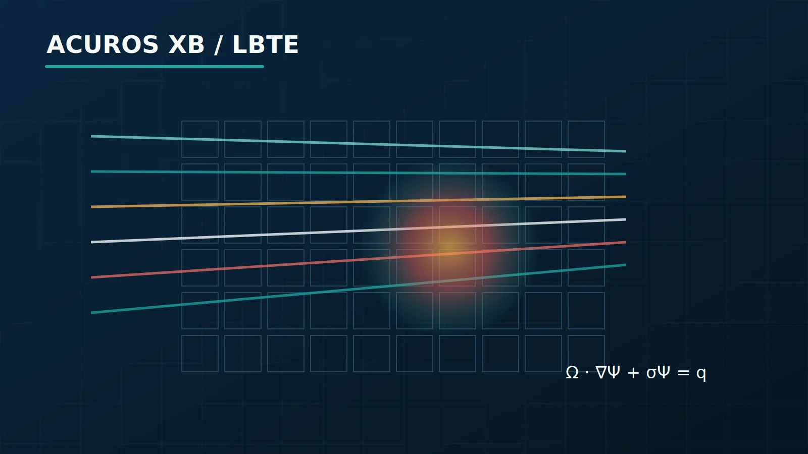
What is LBTE, in clinical language

The linear Boltzmann transport equation is the equation that describes the macroscopic behavior of radiation particles as they propagate and interact with matter. Instead of thinking about “a pre-tabular dose spread across a kernel”, the formulation starts to follow the balance between:

• particles that enter a volume element;
• particles that come out;
• particles removed by interaction;
• particles generated by scattering and secondary production.

In the Eclipsemanual, the central equations appear, for photons and electrons, summarized as follows:

These expressions are less scary when they are translated.

\Psi^\gamma e \Psi^e

Represent the angular fluence of photons and electrons. In practical terms, they describe the number of particles traveling in a certain direction, position and energy.

\Omega \cdot \nabla \Psi

It is the term of streaming: the part of the problem that describes the spatial transport of fluence.

\sigma_t \Psi

It is removal by interaction. As particles pass through the medium, some of them are removed by collisions and other processes.

q

These are the source terms: external particles coming from the head model, scattered photons, electrons produced by photons and electrons generated by other interactions.

\partial_E(S_R \Psi^e)

It is the term that represents the continuous loss of electron energy, including the role of stopping power.

Instead of applying a ready-made deposition recipe, the algorithm balances these flows and interactions to obtain fluence inside the patient. Only then do you convert this into a dose.

The calculation flow of Acuros XB

One of the most useful figures in Varian’s guide is precisely the one that summarizes the calculation sequence. It is already extracted locally:

The manual organizes the process into five steps:

1. creation of the physical map of materials;
2. transporting the source components into the patient;
3. calculation of the fluence of scattered photons;
4. calculation of the fluence of colliding electrons;
5. dose calculation in the desired mode.

This order really helps to separate Acuros XB from vague explanations. The algorithm does not “correct heterogeneities better”; it performs a physically and numerically different chain of operations.

It all starts with the map material

A decisive difference between AAA e Acuros XB It is the role of the image. AAA works with electron density. The Acuros XB works with mass density and material composition. This already puts you in a different universe.

The manual is explicit: Eclipse provides Acuros XB with a material type and mass density in each voxel of the image grid. From there, the algorithm composes macroscopic cross sections for each material.

This part deserves attention because a lot of discussion about algorithms forgets that physics is only as good as the material representation of the patient. There is no point in having a sophisticated solver if the CT to material mapping is poorly solved.

In Acuros XB, the expression for the macroscopic cross section is presented as follows:

In practical terms, this means that the probability of interaction per unit path depends:

• on the mass density of the material;
• of the atomic composition;
• of the microscopic cross sections of the processes involved.

It is this foundation that allows the algorithm to respond more physically in bone, air, lung and dense materials.

CT to material mapping is not bureaucracy

Varian’s guide addresses the CT to material mapping with a level of detail that is worth preserving editorially. The algorithm may stop the calculation if it finds values ​​of HU above the maximum covered by the calibration curve. There is also specific logic for high-density materials, including:

• maximum volume for automatic assignment;
• need for material override in larger volumes;
• extension of the calibration curve for very dense materials.

This excerpt is usually read as an operational detail, but it is conceptually important. Acuros XB only delivers what it promises because it doesn’t treat the patient like climbing water. When the case involves metal, artifact or very dense materials, the user’s responsibility increases, not decreases.

There is also a fine and clinically interesting point: the manual comments that image noise can produce rapid switching between two materials when the calculated mass density is close to the limit between them. This may appear as discrete noise in the dose. This detail is useful because it shows a difference in sensitivity compared to less material-dependent algorithms.

Discretization: the price of the explicit solution

Acuros XB does not resolve LBTE on the ideal continuum. It solves a discretized version of the problem. This means that its characteristic errors are mainly systematic discretization errors, not statistical noise as in Monte Carlo.

The manual divides this discretization into three axes:

Space

The computational volume is subdivided into Cartesian elements of variable size. The algorithm uses adaptive mesh refinement, with finer resolution within the primary volume of interest and coarser resolution outside of it.

This is important because it shows that Acuros XB does not treat the entire scene with the same cost. It focuses computational effort where dose and gradients matter most.

Energy

The algorithm uses the multigroup method to discretize energy. The cross section library includes 25 energy groups for photons and 49 for electrons, although not all are used at lower energies.

Angle

For the spatial transport of scattered particles, Acuros XB uses the discrete ordinatesmethod. Angular space is discretized in a finite set of directions, and the order of quadrature varies with particle and energy.

This part is central to understanding the nature of the algorithm. Acuros XB gains speed over a traditional Monte Carlo because it abandons the stochastic draw of individual stories and replaces this with a structured discretization of transport.

Monte Carlo and Acuros converge to the same physics?

The Varian manual is careful on this point. He claims that both Monte Carlo while explicit LBTE solution methods are convergent and, with sufficient refinement, approximate the same physical solution.

This observation helps dispel two common misconceptions.

The first mistake is to think that Acuros XB is just an “improved analytical” algorithm. It is not. It belongs to the universe of explicit transport solvers.

The second mistake is to treat Monte Carlo as if it were the only legitimate way to get close to real physics. It’s not either. Acuros XB tries to reach the same problem through another numerical path.

What changes between them, in practice, is:

• nature of the dominant error;
• computational cost;
• way of controlling accuracy;
• sensitivity to discretization and material modeling.

What happens to the dose after creep

After solving for electronic creep, the algorithm converts this into dose by a relationship like:

This is where the dose to medium versus dose to water debate takes concrete shape.

When the Acuros XB calculates dose to medium, the energy deposition cross section and density used are those of the local material itself. When it calculates dose to water, it uses the water response to convert the electronic fluence already calculated in the real medium.

Varian’s guide explains this point with a clarity that should be replicated more in clinical discussions. In non-aqueous materials, especially high-density non-biological materials and also in bone, the equivalent volume of water that would receive that dose can be much smaller than the output voxel or a physical detector used in experimental measurements.

This observation changes the way of interpreting results in:

• cortical bone;
• aluminum;
• titanium;
• steel;
• high density implants.

Dose to medium versus dose to water: why this matters

The figure comparing energy deposition ratios e collisional stopping power ratios, also already extracted locally, is one of the best entry points for this topic:

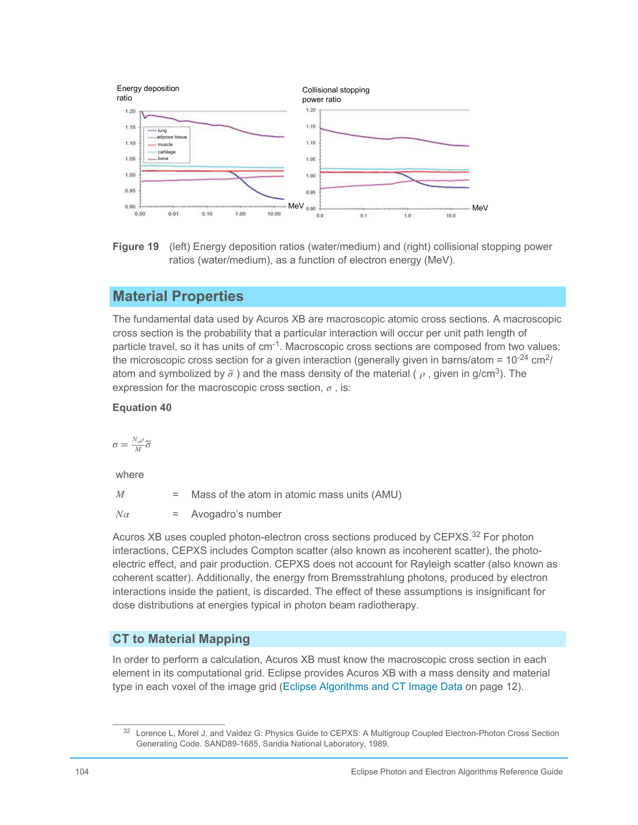
The central point is the following:

• Acuros XB calculates the electronic fluence in the real medium;
• if the user chooses dose to medium, the final conversion respects the local material;
• if you choose dose to water, the conversion uses the water response in that same creep field.

This means that the difference between the two modes is not an interface quirk. It is a difference in physical interpretation of the same calculated fluency.

In clinical practice, this distinction may be small in many soft tissues, but it is no longer irrelevant in bone and non-biological materials. The most common mistake here is to compare two plans or two engines as if they both spoke of exactly the same magnitude.

Where Acuros XB often shows real clinical value

Acuros XB tends to show its gain more clearly when the hypothesis of simple scaling of the medium is no longer sufficient. These include:

• lung and soft tissue reentry;
• air cavities;
• bone-tissue interfaces;
• presence of implants and dense materials;
• small, irregular fields;
• situations where the lateral physics of electronic transport weigh heavily.

In several of these scenarios, the comparison with AAA does not just produce a statistical nuance. It can produce a noticeable change in dose distribution in critical regions.

This is the reason why Acuros XB has established itself in so many services as a preferred option for heterogeneous cases. Not because it “sounds more modern”, but because the physical family it belongs to was designed to better respond to this type of problem.

What Acuros XB can’t solve alone

There is a curious risk when an algorithm gains a reputation for being physically superior: people start to expect responses from it that are independent of the rest of the system. This never happens.

Acuros XB does not correct itself:

• an inadequate CT curve;
• a poorly configured material mapping ;
• a poorly configured beam model bad;
• poorly chosen grid resolution;
• methodologically incorrect comparisons with other engines.

Furthermore, the documentation itself draws attention to situations where high-density materials above the automatic assignment limit require override structured. In other words: the algorithm is more physical, but it also requires more discipline in data preparation.

Acuros XB and AAA: the comparison worth making

Comparing AAA e Acuros XB just as “fast” versus “accurate” impoverishes them both. The best comparison is this:

Question	AAA	Acuros XB
How is the environment treated?	Scaling by electron density and anisotropic kernels	Explicit material mapping with mass density and cross sections
How is the dose constructed?	Convolution/superposition of beamlets	Numerical resolution of transport followed by dose conversion
Dominant error	Limitations of the kernel model and the approximation in strong heterogeneity	Systematic discretization error and dependence on material mapping
Where does it usually gain ground?	Fast and robust clinical flow for a large part of the routine	Strong heterogeneities, implants, difficult interfaces and small fields

This table is more useful than any slogan because it shows that algorithms are not just on different steps of “quality”. They respond to different physical problems with different philosophies.

Where Acuros XB stands in relation to Monte Carlo

This is where mysticism often arises. Acuros XB is not Monte Carlo. But it’s also not just a refined analytical algorithm. It is a deterministic transport solver.

The Varian manual emphasizes that both Monte Carlo and the explicit solution of LBTE, are convergent methods. In many scenarios, they produce very close results. The difference is less in “one being real and the other not” and more in:

• how each one arrives at the result;
• what computational cost does it pay;
• what type of error does it carry;
• how accuracy is controlled.

This point is important because it prevents two symmetric exaggerations:

• reducing Acuros XB to an expensive version of a kernel-based algorithm;
• treat Monte Carlo as the only admissible reference of physical truth.

In the clinic, the correct question is not “which one is more pure”, but “which one solves the relevant problem of this case with the right combination of accuracy, interpretability and flow”.

Conclusion

Acuros XB It matters because it changes the question that TPS can answer. Instead of relying primarily on energy redistribution by pre-built kernels, it numerically solves the transport of photons and electrons in a materially explicit medium. This makes it especially valuable in scenarios where heterogeneity, interfaces and dense materials stop being details and start to dominate the dose behavior.

The algorithm’s gain is not in appearing more sophisticated. It’s about belonging to another physical family. This difference appears in CT to material mapping, in the nature of the errors, in the dose to medium versus dose to water debate and, mainly, in the way the calculation responds when the patient stops behaving like slightly disturbed water.

This does not eliminate the need for rigorous commissioning, careful material configuration and critical reading of results. On the contrary. A more physical engine does not reduce the user’s responsibility; it just shifts the focus of care.

In the next cluster article, this discussion continues precisely at the point where it tends to be oversimplified: what is really at stake when one TPS reports dose to medium and another reports dose to water.

Frequently asked questions

Is Acuros XB Monte Carlo?

No. It deterministically solves a discretized form of the linear Boltzmann transport equation. Monte Carlo samples particle histories; both approaches can converge to similar results when properly implemented.

Why is material mapping important?

Density and composition define the cross sections used in transport. Inadequate mapping can limit the result even when the solver is correct.

Are dose to medium and dose to water interchangeable?

No. The difference may be small in soft tissue and more relevant in bone and other materials. The convention must be documented and kept consistent in comparisons.

Does Acuros always outperform AAA?

There is no universal superiority. Explicit transport is often advantageous in strong heterogeneity, but beam model, grid, version, material mapping, and commissioning remain decisive.

What should commissioning validate?

Open and small fields, heterogeneity, interfaces, grid, monitor-unit calculation, high-density materials, dose convention, and representative clinical workflows.

References

• Fogliata A et al. Dosimetric validation of the Acuros XB advanced dose calculation algorithm. Med Phys. 2011.
• Hoffmann L et al. Clinical validation of the Acuros XB photon dose calculation algorithm. Acta Oncol. 2012.
• Siebers JV et al. Converting absorbed dose to medium to absorbed dose to water. Phys Med Biol. 2000.