Superposition, Clarkson & TERMA in Dose Calculation

Superposition-based dose calculation represents the conceptual leap that separated empirical broad-beam methods from the modern algorithms used in treatment planning systems (TPS). Before reaching convolution itself, however, there is a fundamental intermediate step: separating the primary and scattered radiation components — formalized by Clarkson’s method — and quantifying the total energy released in the medium, expressed through the concept of TERMA. This article traces that trajectory, from angular scatter integrations to the full convolution/superposition kernel formulation, as described in the Handbook of Radiotherapy Physics (2nd edition). For a panoramic view of all algorithms from empirical to Monte Carlo, see our complete guide to photon dose calculation algorithms.

Clarkson’s Method: Primary-Scatter Separation

The core idea behind Clarkson’s method is to separately compute the primary and scattered dose at any point of interest $P$. The primary component depends only on attenuation along the source-to-point axis, while the scattered component depends on the entire field geometry — its shape, size, and proximity to point $P$.

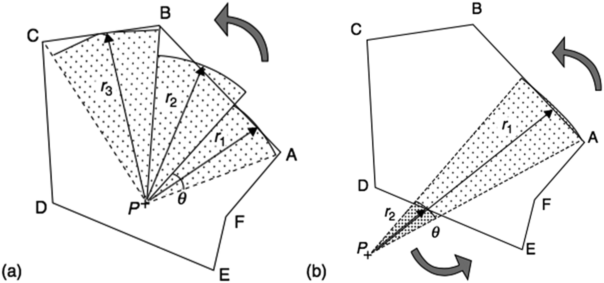
The irregular field is divided into $n$ angular sectors centred on $P$. Each sector $i$ has angular width $\Delta\theta_i$ and radius $r_i$ (measured to the field edge). The scatter is then summed over all sectors using tabulated scatter-air ratios (SARs):

$$D_S(x,y,z) = D_A(z) \times \sum_i S(z, r_i) \frac{\Delta\theta_i}{2\pi}$$

Where:

• $D_A(z)$ is the dose “in air” (without attenuation) at position $(0,0,z)$
• $S(z, r_i)$ is the scatter-air ratio for depth $z$ in a circular field of radius $r_i$
• $\Delta\theta_i / 2\pi$ is the angular fraction of the full circle represented by the sector

The primary component uses the zero-area TAR — a mathematical abstraction representing pure attenuation without scatter. In practice, TAR$_0(z)$ cannot be measured directly; it is obtained by extrapolating TARs for small field sizes back to zero or by measurements under scatter-free conditions at large source-to-detector distances.

$$D_P(x,y,z) = D_A(z) \times \text{TAR}_0(z) \times f(x,y)$$

Here $f(x,y)$ is the off-axis factor in air correcting for the beam profile. The total dose is simply:

$$D(x,y,z) = D_P(x,y,z) + D_S(x,y,z)$$

When point $P$ lies outside the field, the same summation works: sectors traversed right-to-left (A to B) receive positive sign, left-to-right (D to E) negative — retaining only the contribution from inside the field.

2D Integration and Correction for Modulated Fields

Classical Clarkson assumes a flat surface and uniform primary fluence. In clinical practice, the patient surface is oblique and irregular, and the primary beam may be modulated by wedge filters, compensators, or multi-leaf collimators (MLCs). The solution lies in extending to 2D pencil-beam scatter integration:

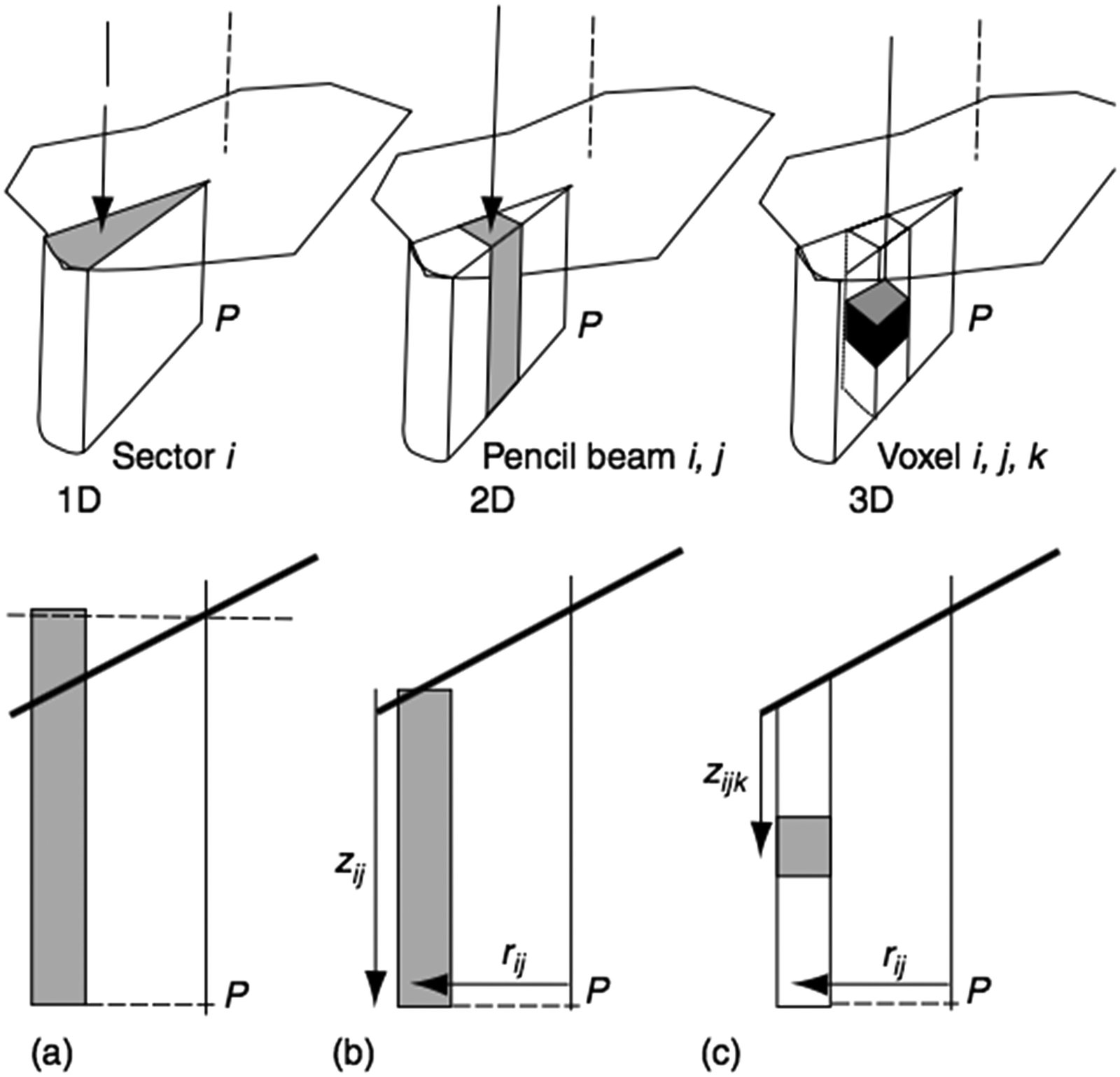
Each scattering element is referenced to a polar coordinate system centred on the calculation point $P$, at distance $r_{ij}$ along the radius defined by angle $\theta_i$, with tissue thickness $z_{ij}$:

$$\Delta S_{ij}(z_{ij}, \theta_i, r_{ij}) = \frac{\Delta\theta_i}{2\pi} \times \left[ S(z_{ij}, r_{ij} + \Delta r) – S(z_{ij}, r_{ij}) \right]$$

During integration over the field area, each pencil beam is weighted by the local primary fluence at point $ij$. This extension yields satisfactory results even for MLC-based IMRT (Papatheodorou et al. 2000), since surface obliquity and intensity modulation are explicitly accounted for.

Attempts to go further — 3D integrations such as the dSAR method (Beaudoin 1968; Cunningham 1972) — encountered problems with the complex behaviour of multiple scattering and were partially abandoned. The delta-volume method (Wong and Henkelman, 1983), dTAR (Kappas and Rosenwald, 1986b), and improved ETAR (Redpath and Thwaites, 1991) brought refinements, but all share a fundamental limitation: they assume the secondary electron path length is negligible.

Extension to Higher Energies: Mini-Phantom and TPR

As photon energy increases, the concept of dose “in air” loses practical relevance. The build-up caps required for electronic equilibrium become too large, and the attenuation and scatter within them cannot be ignored. The TAR must be replaced.

The solution came with the mini-phantom concept: primary component attenuation is represented by the tissue phantom ratio measured in a mini-phantom, TPR$(z, \text{ESQ}_{\text{mini}})$, where ESQ$_{\text{mini}}$ is the equivalent square corresponding to the mini-phantom geometry. The SAR is replaced by SAR$’$, obtained from:

$$\text{SAR}'(z, \text{ESQ}_z) = \text{TAR}'(z, \text{ESQ}_z) – \text{TPR}(z, \text{ESQ}_{\text{mini}})$$

With TAR$’$ defined as:

$$\text{TAR}'(z, \text{ESQ}_z) = \text{TPR}(z, A_z) \frac{S_p(z_{\text{ref}}, \text{ESQ}_z)}{S_p(z_{\text{ref}}, \text{ESQ}_{\text{mini}})}$$

Where $S_p$ is the phantom scatter correction factor. The “in-air” reference dose $D_A$ is replaced by the dose in the mini-phantom at depth $z_{\text{ref}}$ for the current collimator opening $A$, derived through the internal calibration process.

These primary-scatter separation methods yield acceptable results in many clinical situations for fields larger than ESQ$_{\text{mini}}$ in water-like media (Knöös et al. 2006). However, they fail where electronic equilibrium is lacking: field edges, inhomogeneity boundaries, small fields in high-energy beams through lung (Mohan and Chui, 1985; Mackie et al., 1985; AAPM, 2004). This limitation motivated the transition to methods based on superposition of energy deposition kernels.

The Superposition Principle and Kernel Convolution

The idea of using kernel convolution/superposition for dose calculation was independently proposed by several groups in 1984: Ahnesjö, Boyer and Mok, Chui and Mohan, Mackie and Scrimger. The concept is elegant in its generality.

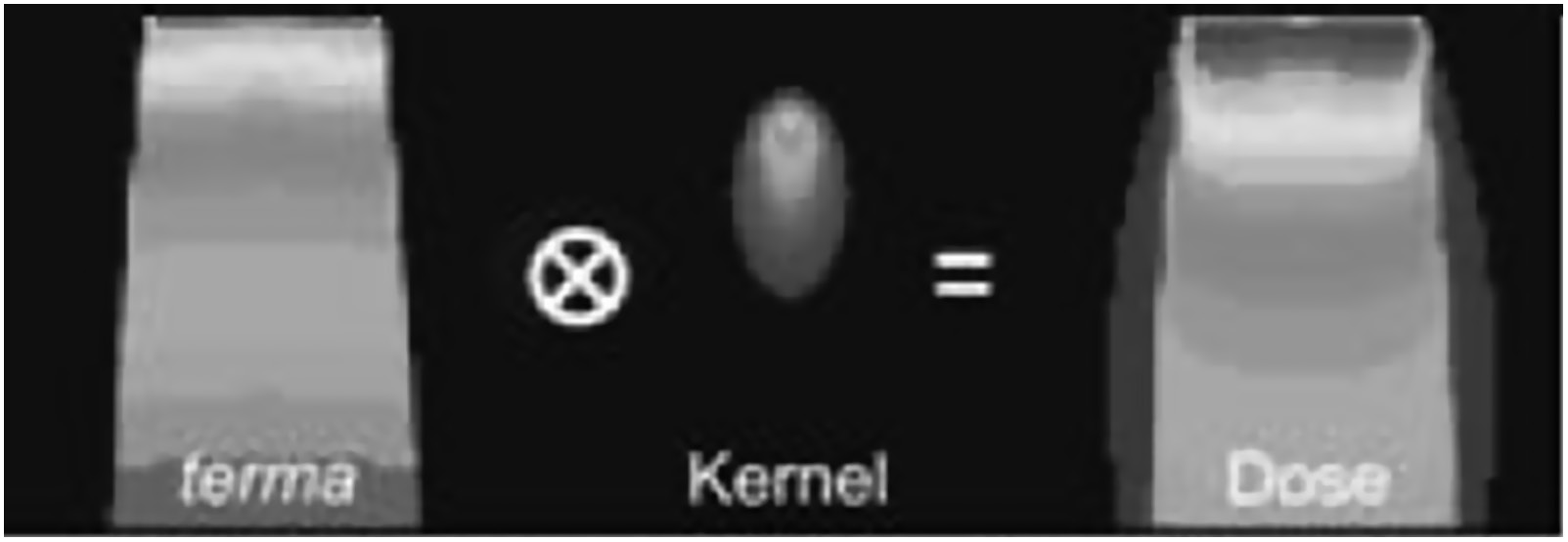
For a homogeneous medium, the dose at point $P$ at position $\mathbf{r} = [x, y, z]$ is given by:

$$D(\mathbf{r}) = \iiint \Psi(\mathbf{r}’) \frac{\mu}{\rho}(\mathbf{r}’) \, K(\mathbf{r} – \mathbf{r}’) \, dV’$$

Where:

• $\Psi(\mathbf{r}’)$ is the energy fluence (J m$^{-2}$) at point $P’$ at position $\mathbf{r}’ = [x’, y’, z’]$
• $\mu/\rho(\mathbf{r}’)$ is the mass attenuation coefficient (m$^2$ kg$^{-1}$) at $P’$
• $\Psi(\mathbf{r}’) \cdot \mu/\rho(\mathbf{r}’)$ is the TERMA — total energy released per unit mass from $dV’$ (J kg$^{-1}$ or Gy)
• $K(\mathbf{r} – \mathbf{r}’)$ is the energy deposition point kernel, representing the fraction of energy released at $dV’$ deposited at $P$

The integration runs in 3D over the patient volume. Mathematically, if the kernel is spatially invariant, the operation is a convolution — allowing the use of Fourier transforms to speed up computation. When the kernel varies spatially (as in heterogeneous media), the operation is a superposition, more computationally demanding but physically more accurate.

For clinical polyenergetic beams, the general formulation requires additional integration over the energy bins of the local beam spectrum, with $\Psi$ replaced by the energy fluence differential in energy, and both $\mu/\rho$ and $K$ being energy-dependent. Boyer et al. (1989) and Zhu and Van Dyk (1995) demonstrated that a limited number of bins suffice.

Energy Fluence and Source Modelling

Dose calculation by convolution requires two fundamental inputs: the energy fluence (or TERMA) at each point $P’$ and the deposition kernels around $P’$. Determining the fluence is a two-step process: modelling the incident fluence at the patient surface and then transporting it through the medium.

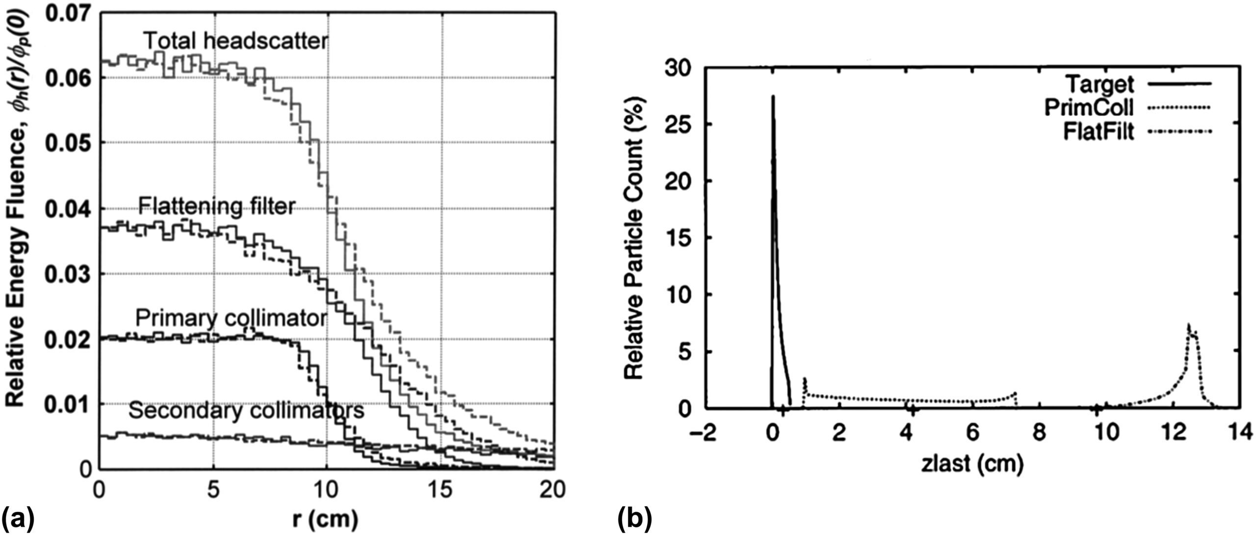
In a linear accelerator, incident photons come primarily from bremsstrahlung emitted from the target. However, typically a few percent are scattered from the flattening filter and, to a lesser extent, from the inner surfaces of the primary and secondary collimators. This extrafocal contribution has an effective source position downstream of the physical target and a bell-shaped profile extending beyond the geometrical field limits.

For flattening filter free (FFF) beams, the extrafocal contribution is smaller and the model can be simplified (Kry et al. 2010; Almberg et al. 2012). For conventional beams, the source model typically combines multiple extended sources — target, primary collimator, flattening filter — integrated over the parts of the head visible from the calculation point (Ahnesjö 1994; Sharpe et al. 1995; Fippel et al. 2003).

Fluence modification at the field edge and beneath the beam-shaping devices is based on geometrical considerations complemented by transmission calculation through the main collimator, blocks, or MLC. With IMRT development, accurate modelling of individual MLC leaf transmission became critical (Tyagi et al. 2007). Results are stored as 2D initial fluence maps, modifiable by correction matrices for each beam-limiting or modifying device.

TERMA: Total Energy Released per Unit Mass

The incident fluence must be transported through the patient by ray tracing along paths diverging from the source position, applying inverse-square-law correction and tissue attenuation between the patient surface and $P’$.

For a monoenergetic beam of energy $E$, the primary radiation attenuation at depth $z’ = \sum_i \Delta z_i$ is calculated as (Ahnesjö et al. 1987):

$$\text{Attenuation} = e^{-\sum_i \left(\frac{\mu}{\rho}\right)_{E,i} \rho_i \Delta z_i}$$

Where $\rho_i$ is the mass density of voxel $i$ and $(\mu/\rho)_{E,i}$ is the mass attenuation coefficient at voxel $i$ for energy $E$.

For polyenergetic beams, computing dose as the weighted sum of each energy bin would be computationally prohibitive (Hoban 1995). A more effective approach uses a single pre-calculated polyenergetic kernel and computes attenuation with effective coefficients $\mu_{\text{eff}}$ averaged according to the spectral bin energy fluence weights. Spectral modification with depth (beam hardening) is handled by exponentially attenuating each component with its own coefficient (Hoban et al. 1994). Additional linear corrections can be applied to $\mu_{\text{eff}}$ for depth hardening (Papanikolaou et al. 1993; Ahnesjö et al. 2005) and off-axis softening (Tailor et al. 1998).

The resulting $\mu/\rho$ values at each point $P’$ are stored in a 3D look-up table and multiplied by the local energy fluence to yield the 3D TERMA distribution (Metcalfe et al. 1990). TERMA is, therefore, the “available energy map” that will be redistributed by the deposition kernels.

In-Water Energy Deposition Kernels

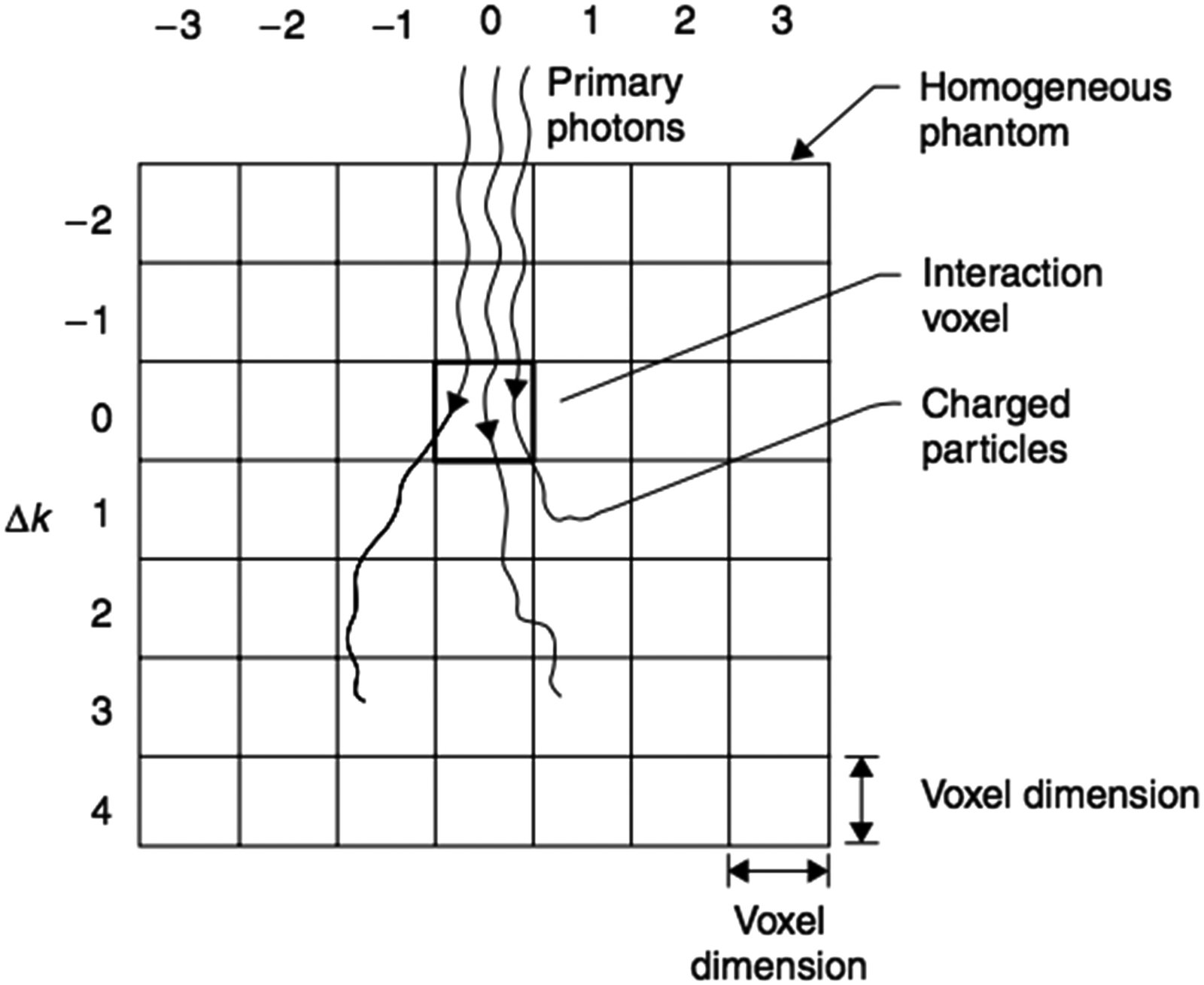
The kernels $K$ in the convolution equation are determined by Monte Carlo simulation in a water phantom, forcing primary photon interactions at the origin voxel (Mackie et al. 1988; Mohan et al. 1986; Ahnesjö et al. 1987). Spherical geometry with polar coordinates is the standard choice, with radial and angular intervals providing accurate energy deposition representation at any distance from the interaction point.

These kernels can be decomposed into a primary kernel $K_p$ (energy deposited by charged particles from primary photons) and a scatter kernel $K_s$ (energy deposited by all charged particles from scattered photons, including bremsstrahlung and annihilation radiation). The kernel $K$ is normalized as the fraction of incident energy per unit volume (cm$^{-3}$), satisfying:

$$\iiint_{\infty} K(\mathbf{r}) \, dV \approx 1$$

The component integrals follow fundamental relationships (Mackie et al. 1988; Boyer et al. 1988):

$$\iiint_{\infty} K_p(\mathbf{r}) \, dV = \frac{\mu_{\text{en}}}{\mu}$$

$$\iiint_{\infty} K_s(\mathbf{r}) \, dV = \frac{\mu – \mu_{\text{en}}}{\mu}$$

Where $\mu$ is the linear attenuation coefficient and $\mu_{\text{en}}$ is the linear energy absorption coefficient. These relationships serve for kernel verification and for applying corrections due to beam quality variations.

For clinical polyenergetic beams, the most effective approach is to generate polyenergetic kernels by weighted addition of pre-calculated monoenergetic kernels according to the normalized incident energy fluence spectrum. Since the spectrum changes with depth and lateral position (beam hardening), Liu et al. (1997d) proposed pre-calculating polyenergetic kernels at different depths (typically three) and interpolating between them.

Clarkson vs Convolution/Superposition: When to Use Each?

Feature	Clarkson / Primary-Scatter Separation	Convolution/Superposition of Kernels
Physical principle	Empirical primary + scatter separation with tabulated SARs	3D integration of TERMA with MC energy deposition kernels
Heterogeneity handling	Correction factors (Batho, ETAR); assumes negligible electron path	Density-scaled kernels; implicitly models electron transport
Field edge accuracy	Limited for small fields and lung/tissue interfaces	Superior, especially with anisotropic kernels
Modulated fields (IMRT)	Possible with 2D extension (pencil scatter)	Naturally compatible via 2D fluence maps
Computational speed	Fast (tables + summations)	Slower (3D convolution); accelerable with FFT
Current clinical use	Largely superseded, except legacy systems	Basis of modern commercial algorithms (CCC, AAA, Pinnacle)

Comparative table based on the Handbook of Radiotherapy Physics, 2nd Ed.

Clinical Application of Modified Clarkson: Independent Monitor Unit Verification

Although primary-scatter separation methods have been largely superseded in modern TPS, the Modified Clarkson algorithm retains a fundamental clinical role: independent verification of monitor unit (MU) calculations. Radiotherapy quality assurance programs require that the TPS-generated MU calculation be checked by a second method, preferably based on an independent algorithm and independent data. The computational speed and well-understood physical basis of Modified Clarkson make it ideal for this double-check function.

The RTConnect software, developed by RT Medical Systems, uses precisely this approach: it implements the Modified Clarkson algorithm for independent MU verification in 3D conformal fields and MLC-based techniques. The calculation accounts for primary-scatter separation with equivalent SARs, tray corrections, wedge filters, and off-axis factors, providing a fast and reliable check that complements the primary TPS result. This Clarkson-based verification methodology is well documented in the literature, as described in the IAEA technical article on Clarkson-method MU verification.

In clinical practice, using an independent double-check system such as RTConnect is not merely good practice — it is a requirement of accreditation programs and quality audits. The discrepancy between the TPS calculation and the independent verification serves as an indicator of potential data entry errors, plan configuration issues, or algorithmic limitations under specific conditions.

Primary-scatter separation methods were historically important and still yield acceptable results in water-like media for regular fields. But the demand for accuracy in heterogeneities, small fields, and IMRT pushed the state of the art towards kernel convolution/superposition — which in turn paved the way for commercial algorithms such as Collapsed Cone Convolution (CCC) and clinical Monte Carlo.

The transition from Clarkson to convolution was not merely a change of method; it was a paradigm shift. Clarkson operates on tabulated empirical data — TARs, SARs, measured profiles. Convolution operates on fundamental physical quantities — fluence, TERMA, kernels derived from first principles via Monte Carlo. This physical basis makes convolution/superposition methods inherently more generalizable and reliable outside calibration conditions.

For a deeper dive into deposition kernels and the Collapsed Cone Convolution algorithm specifically, follow the upcoming articles in this series. If you work with treatment planning and DVH recommendations, understanding these foundations is indispensable for critically evaluating your TPS results.