
Introduction to Proton Therapy and Monte Carlo
Proton therapy has established itself as one of the most precise external beam radiotherapy techniques, leveraging the Bragg peak to concentrate dose within the target volume with a sharp distal falloff. However, the very precision that makes protons so clinically attractive also demands dose calculation models of matching accuracy — and that is precisely where Monte Carlo becomes indispensable.
Unlike photons — whose interactions are dominated by Compton scattering and the photoelectric effect — protons lose energy through ionizations, multiple Coulomb scattering, and nuclear interactions. Each process relies on distinct physics models, cross sections, and material constants that analytical algorithms simplify considerably. Monte Carlo tracks each particle individually and applies real probability distributions for every interaction, achieving dose accuracy of approximately 1%–2%, compared to potentially larger uncertainties from pencil beam algorithms.
For a comprehensive overview of all Monte Carlo applications, check our complete guide on Monte Carlo in Radiotherapy.
Beam Delivery: Passive Scattering vs. Beam Scanning
Two fundamental paradigms exist for proton delivery, and the complexity of Monte Carlo simulation varies dramatically between them.
In passive scattering, the beam is broadened by a double-scattering system and modulated by a rotating modulator wheel to create the spread-out Bragg peak (SOBP). Apertures confine the field laterally, and range compensators shape the distal edge to conform to the target shape. Each field has a unique treatment head configuration — energy, scatterers, modulator, aperture, and compensator — making phase spaces hardly reusable and simulations computationally expensive.
In beam scanning, two magnets deflect individual pencil beams in $x$ and $y$ directions while energy is adjusted layer by layer before the beam enters the room. No patient-specific hardware is mandatory (though apertures may be used to sharpen the penumbra). This simplicity enables analytical source models and reusable phase spaces, making Monte Carlo feasible for routine clinical use in scanning.
As a rule of thumb, approximately 1% of primary protons undergo a nuclear interaction per centimeter of beam range. These interactions generate a nuclear halo around each pencil beam, with significant contributions when multiple beamlets overlap. Monte Carlo simulations must predict this halo correctly for accurate dose — something analytical algorithms typically neglect or oversimplify.
Beam Characterization at Treatment Head Entrance
The starting point of any Monte Carlo simulation in proton therapy is the beam parameterization at the treatment head entrance. Key variables include: beam energy ($E$), energy spread ($\Delta E$), spot size ($\sigma_x$, $\sigma_y$), and angular distribution ($\sigma_{\theta x}$, $\sigma_{\theta y}$).
Typical proton beam spot sizes range from 2–8 mm in $\sigma$, while the angular spread is on the order of 2–5 mm-mrad for beams from a cyclotron. For passive scattering, angular spread at the head entrance has little influence on the exit beam since the scattering material dominates. For beam scanning, however, the correlation between particle position within the beam spot and its angular momentum must be modeled — a full phase-space parameterization can be derived from the magnetic beam steering system or by fitting measured data.
The energy spread from a cyclotron is typically less than 1% ($\Delta E/E$), while synchrotrons can extract beams with energy spread two orders of magnitude lower. Measuring beam energy with sufficient accuracy involves analyzing Bragg curves in water or elastic scattering techniques.
Monte Carlo Modeling of the Treatment Head
The fidelity required when modeling the treatment head depends on the simulation purpose. For patient dose calculation, only the main beam-shaping devices need to be included. In beam scanning, these are the scanning magnets and any apertures. In passive scattering, the full double-scattering system, modulator wheel, aperture, and compensator must be modeled.
The modulator wheel — a rotating mechanical component with tracks of varying thickness — can be handled in Monte Carlo either as multiple static geometries or using 4D techniques that dynamically change the geometry. Common track materials include polyethylene (lexan) and lead; a 10% variation in their density can cause range changes on the order of 1 mm.
Apertures must be modeled explicitly due to secondary radiation and edge-scattering effects. Compensators with irregular geometry require CAD import or boundary point definition. For simulating scanning patterns, 4D Monte Carlo techniques allow studying the details of beam delivery parameters.
Monte Carlo is also used to design prompt gamma detectors for range verification, optimize image reconstruction for proton CT, and study scattering in multi-leaf collimators as alternatives to patient-specific apertures. Simulations can further support clinical QA programs by reducing the need for extensive experimental studies while defining beam parameter tolerances.
Phase Spaces and Source Models
A phase space records the type, energy, direction, and position of typically tens to hundreds of millions of particles at a plane perpendicular to the beam central axis. For passive scattering, phase spaces at the treatment head exit are of limited use — each field has a unique configuration. For beam scanning, however, variations are limited to energy and magnet settings, making phase spaces highly reusable.
Beyond phase spaces, analytical source models are viable for beam scanning: each pencil beam is parameterized by position ($x$, $y$), energy, weight, divergence, and angular spread, derived from fluence measurements in air and depth-dose curves in water. Secondary particles generated in the treatment head can typically be neglected.
An important caveat: characterizing each beamlet with a simple Gaussian fluence distribution overestimates the central fluence because it ignores the halo from large-angle scattered protons. A second Gaussian in the formalism is usually needed for correction. This has direct implications for clinical Monte Carlo feasibility — since the bulk of computation time in passive scattering is spent tracking particles through the treatment head, beam scanning simulations are orders of magnitude more efficient.
CT Conversion and Material Assignment
For Monte Carlo dose calculation, each CT voxel must be converted to material composition, mass density, and ionization potential. Unlike analytical algorithms that use relative stopping power, Monte Carlo operates with explicit material properties.
CT conversion schemes group tissues into 5–30 groups sharing the same material composition. However, soft tissues in the 0–100 Hounsfield unit (HU) range are poorly distinguished — similar CT numbers can represent distinctly different elemental compositions. A change in conversion method can influence beam range by 1–2 mm in head and neck treatments.
| Conversion Parameter | Typical Impact | Notes |
|---|---|---|
| Elemental composition | Most significant effect | Differences in H, C, O, Ca between methods (Schneider vs Rogers) |
| Mass density | Minor role in target region | More relevant in bone and interfaces |
| Mean excitation energy | 5%–15% uncertainty | Directly impacts range prediction |
| Dual-energy CT | Improves material assignment | Provides two attenuation maps for more accurate compositions |
Source: Monte Carlo Techniques in Radiation Therapy (2nd ed., CRC Press, 2022)
Mean excitation energies for tissues carry uncertainties of 5%–15%, directly reflected in range prediction. Dual-energy CT significantly improves material assignment by providing two different attenuation maps, enabling more accurate determination of relative electron densities and effective atomic numbers.
Absolute Dose and Dose-to-Water vs. Dose-to-Tissue
Planning systems prescribe dose in Gy per GigaProtons or in cGy per monitor unit (MU). Monte Carlo can directly simulate the charge collected in the treatment head transmission ionization chamber — but this requires many histories and a detailed nozzle model. Alternatively, one can relate the number of protons at the head entrance to the dose in an SOBP in water, an equivalent method when the head model is accurate.
A fundamental distinction: analytical algorithms calculate dose-to-water (clinical experience, measurements, and constraints are based on this), while Monte Carlo inherently calculates dose-to-tissue. The difference can reach 10%–15% in bony anatomy but is on the order of ~2% in soft tissues. In practice, a retroactive conversion using energy-independent relative stopping powers achieves accuracy within ~1%.
Nuclear Interactions and Dose Impact
Nuclear interactions contribute well over 10% of the total dose, particularly in the entrance region of the Bragg curve, where secondary protons cause a dose buildup through predominantly forward emission. The fluence reduction of the primary beam due to nuclear collisions is also notable.
The average energy at the Bragg peak is about 10% of the initial energy. Nuclear interaction cross sections peak at approximately 20 MeV and decrease sharply, making the nuclear contribution negligible near the pristine Bragg peak position. For an SOBP, however, contributions proximal to the peak remain relevant, causing a tilt of the SOBP dose plateau if neglected.
For patient dose calculations, only secondary protons from proton-nuclear interactions need to be tracked — the energy of other secondary particles can be deposited locally when their projected range is smaller than the voxel size. Learn more about these principles in our article on Monte Carlo fundamentals in radiotherapy.
Monte Carlo vs. Analytical Algorithms: Clinical Differences
Most proton therapy treatment plans still rely on analytical pencil beam algorithms, and Monte Carlo has been used both for validation and commissioning. The differences become clinically significant in regions with pronounced tissue heterogeneities.
Range Prediction Differences
The range of a clinical proton field is defined as $R_{90}$ — the position of the 90% dose level in the distal falloff of the SOBP. Globally, range differences between analytical and Monte Carlo are small (both commissioned in water). Locally, however, significant discrepancies occur where the beam traverses heterogeneities.
In clinical practice, range margins of approximately 3.5% + 1 mm are commonly applied. With Monte Carlo, these margins could be uniformly reduced to 2.4% + 1.2 mm regardless of the patient’s geometric complexity. For homogeneous geometries (such as liver), margins can be as low as 2.7% + 1.2 mm, but for geometries with lateral inhomogeneities (head and neck, lung), the analytical approach may require up to 6.3% + 1.2 mm.
| Geometry | Analytical Margin | Monte Carlo Margin |
|---|---|---|
| Homogeneous (liver) | 2.7% + 1.2 mm | 2.4% + 1.2 mm |
| Lateral inhomogeneities (head/neck, lung) | Up to 6.3% + 1.2 mm | 2.4% + 1.2 mm |
| Generic (current practice) | 3.5% + 1 mm | 2.4% + 1.2 mm |
Source: Monte Carlo Techniques in Radiation Therapy (2nd ed., CRC Press, 2022)
Dose Prediction Differences
The greater multiple scattering predicted by Monte Carlo causes a broadening of the dose distribution and consequently lower doses in the medium-to-high dose region. Target dose from Monte Carlo is generally slightly lower than predicted by analytical algorithms. For head and neck and lung patients, mean target dose differences can reach 4%. In breast and liver, differences remain around 2%. Small fields are even more sensitive.
Extreme cases include metallic implants — such as dental implants in head and neck cancer patients — which cause significant dose perturbations typically not predicted accurately by analytical algorithms due to their high-Z nature. For details on dose calculation in complex scenarios, see our article on Monte Carlo patient dose calculation.
Clinical Implementation and Monte Carlo-Based Planning
Implementing Monte Carlo in a proton therapy clinic involves transferring planning system information to the Monte Carlo code via a DICOM-RTion interface. Major proton centers already operate in-house Monte Carlo systems for dose verification or research. The interface must translate gantry angle, couch angle, isocenter position, voxel dimensions, and prescribed dose.
For inverse planning with Monte Carlo (IMPT), computational requirements are stricter — each possible beamlet must be pre-calculated with high statistical precision before optimization. Fast Monte Carlo simulation tools are essential. In practice, optimization can be based on the analytical algorithm with Monte Carlo used only for fine-tuning or at limited checkpoints during the iterative process.
Major treatment planning system vendors are currently working toward incorporating Monte Carlo. Improvements in both computational efficiency of the software and hardware have made routine use feasible.
Advanced QA with Monte Carlo in Proton Therapy
Quality assurance in proton therapy benefits enormously from Monte Carlo in several ways:
First, simulations can define tolerances for beam parameters. By systematically varying input parameters and observing the impact on dose distributions, acceptable limits for spot size, energy, and head alignment are established without the need for extensive measurements.
Second, Monte Carlo is used to recalculate plans from treatment log files, enabling dose-delivery verification that considers what was actually delivered, not just what was planned.
Third, range verification applications use Monte Carlo simulations to model prompt gamma emission — photons emitted during nuclear interactions that carry information about the Bragg peak position in vivo. Monte Carlo is essential for designing detectors and optimizing reconstruction algorithms.
Fourth, simulations of LET distributions (linear energy transfer) are fundamental for radiobiological considerations. LET varies considerably along depth in proton therapy, with direct implications for relative biological effectiveness (RBE). Monte Carlo enables mapping these distributions with spatial precision that experimental measurements can hardly achieve.
Finally, track structure simulations at the nanoscale — using extensions like TOPAS-nBio based on Geant4-DNA — allow investigating DNA damage and ionization clustering in subcellular volumes, connecting particle transport physics directly to radiobiology.
Monte Carlo Codes for Proton Therapy
Several codes are available for proton therapy simulations:
| Code | Base | Key Features |
|---|---|---|
| TOPAS | Geant4 | User-friendly interface, no programming required; NCI-supported |
| GATE | Geant4 | Framework for radiotherapy and imaging applications |
| GAMOS | Geant4 | Simulation framework with simplified interface |
| PTsim | Geant4 | Dedicated to proton therapy |
| FICTION | FLUKA | Radiotherapy-focused wrapper for FLUKA |
| FLUKA | Standalone | Multipurpose code with detailed nuclear models |
| MCNPX | Standalone | Extensive cross-section libraries |
| VMCpro | Standalone | Speed-optimized for proton therapy |
| Shield-Hit | Standalone | Focused on heavy ions and protons |
Source: Monte Carlo Techniques in Radiation Therapy (2nd ed., CRC Press, 2022)
TOPAS deserves special mention: designed within NCI’s ‘Informatics Technologies for Cancer Research’ initiative, it allows non-experts and non-physicists to perform complex Monte Carlo simulations without programming. For more on codes and applications across modalities, see our article on Monte Carlo for ion beams.
Computational Efficiency and Future Outlook
Monte Carlo efficiency in proton therapy depends on several factors: number of histories, step size (limited by CT voxel size, typically 0.5–5 mm), and tracking algorithms in voxelized geometry. Geometry re-segmentation techniques and dose distribution denoising (smoothing) can reduce the required number of histories, though they must be applied with caution — smoothing methods tend to soften dose gradients, which is especially problematic in proton therapy.
The desired statistical uncertainty is typically less than 2% in the target volume. Fewer protons are needed to achieve this precision compared to photons, since protons are directly ionizing with higher LET. CT grid interpolation to larger voxels is not recommended before the simulation (averaging material compositions is ill-defined), but resampling can be done after dose calculation with proper volume-weighted averaging.
With simultaneous evolution of software (more efficient codes, GPUs) and hardware, Monte Carlo for proton therapy is firmly progressing toward becoming the standard for dose calculation — progressively replacing the analytical algorithms that dominated the past decades. To understand how artificial intelligence may further accelerate this transition, see our article on AI and the future of Monte Carlo in radiotherapy.