The pencil beam algorithm, the Fast Pencil Beam, and the AAA (Analytical Anisotropic Algorithm) have dominated commercial treatment planning systems for decades. While the pencil beam decomposes the clinical beam into narrow elementary beams and convolves them with incident fluence, the Fast Pencil Beam trades some of that accuracy for dramatic computational speed in optimization loops. The AAA advances the original concept by separately treating longitudinal and lateral components with density-based anisotropic scaling. This article provides an in-depth analysis of all three methods — from mathematical foundations to clinical limitations in heterogeneous media — based on the Handbook of Radiotherapy Physics (2nd Ed., CRC Press).
In This Article
- 1. The Pencil Beam Principle for Photons
- 2. Kernel Determination
- 3. Practical TPS Implementations
- 4. Limitations in Heterogeneous Media
- 5. Fast Pencil Beam: Speed for Optimization
- 6. AAA in Eclipse: Beyond the Pencil Beam
- 7. AAA Performance and Limitations
- 8. Electron Pencil Beam: Fermi–Eyges Model
- 9. Proton Pencil Beams
- 10. Commercial Algorithm Comparison
The Pencil Beam Principle for Photons
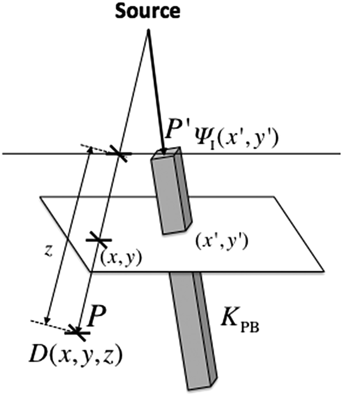
The central idea is straightforward: decompose the clinical beam into a set of narrow elementary beams (“pencils”) and sum their dose contributions at each calculation point. The dose at point $P(x,y,z)$ results from integrating pencil beam kernels $K_{PB}$ weighted by the incident primary energy fluence $\Psi_I$ over the field area:
$$D(x,y,z) = \iint \frac{\mu}{\rho} \Psi_I(x’,y’) \, K_{PB}(x-x’, y-y’, z) \, dx’ \, dy’ \quad (28.32)$$
Where:
- $\Psi_I(x’,y’)$ is the incident energy fluence at $P’$ (J m⁻²)
- $\mu/\rho$ is the mass attenuation coefficient (m² kg⁻¹) of the medium at $P’$
- $(\mu/\rho)\Psi_I(x’,y’)$ is the TERMA — total energy released per unit mass (J kg⁻¹ or Gy)
- $K_{PB}(x-x’, y-y’, z)$ is the pencil beam kernel, representing the fractional energy deposition per unit mass at $P$ due to primary energy fluence entering at $P’$
The key difference between the pencil beam and primary-scatter separation (Clarkson method) lies in what is integrated. In the pencil beam, the “pencil” carries all the energy deposited at a distance — from both secondary electrons and scattered photons. In the superposition approach with Clarkson, only the scatter component is scanned over the field area.
This makes the pencil beam naturally suited for modeling incident intensity variations — whether from wedge filters, compensators, or dynamic intensity modulation (IMRT). Off-axis spectral variations can also be accommodated by adjusting the pencil beam quality at each entrance position.
Kernel Determination
The pencil beam kernel is the heart of the method. Several approaches exist, and the choice directly impacts clinical accuracy.
Direct Monte Carlo Kernels
Mohan and Chui (1987) performed direct Monte Carlo calculations using EGS4 to generate monoenergetic and polyenergetic pencil beam kernels for cobalt-60, 6 MV and 18 MV beams. They demonstrated that the method relied only on fundamental physics principles, without empirical assumptions or arbitrary analytical functions to describe the source distribution.
Ahnesjö’s Analytical Model
Ahnesjö et al. (1992b) presented a complete clinical pencil beam model using polyenergetic kernels obtained from in-depth convolution of Monte Carlo-derived energy deposition point kernels. These kernels could be represented analytically with high accuracy as a sum of two exponentials over the radius:
$$K_{PB}(r,z) = \frac{A_z \, e^{-a_z r}}{r} + \frac{B_z \, e^{-b_z r}}{r} \quad (28.33)$$
Where $r$ is the cylindrical radius from the pencil beam axis, and $A_z$, $a_z$, $B_z$, $b_z$ are depth-dependent fitting parameters. The $r$ denominator (rather than $r^2$ as in point kernels) compensates for geometric dispersion from an infinite line source.
For all dose components except photon scatter, the Ahnesjö model handles tissue variations and patient contour through depth scaling — using pencil beam parameters at the radiological depth (water-equivalent depth). For the scatter dose, geometric depth parameters are used followed by a specific scatter correction factor.
Practical TPS Implementations
In homogeneous media, pencil beam kernels can be assumed position-invariant, turning Equation 28.32 into a true convolution. The fast Fourier transform (FFT) can then dramatically speed up computation — a strategy successfully exploited by Boyer (1984) and Mohan and Chui (1987).
Mohan and Chui demonstrated the power of the pencil beam method for irregular fields in a uniform medium with a flat surface. For a 15 MV beam, despite neglecting off-axis spectral variations, they achieved excellent agreement with measurements because the Monte Carlo-generated pencil beams automatically accounted for the transport of scattered photons and secondary electrons.
Bortfeld et al. (1993) maximized efficiency by decomposing the kernel into three separate terms, reducing the required number of 2D convolutions, and employing the fast Hartley transform. Storchi and Woudstra (1996) developed a model parameterized from limited experimental data, introducing both scatter and boundary kernels. Deviations were less than 2% for rectangular and irregular fields, except for 45° wedges or under blocks (4–5%). This algorithm was incorporated into the Cadplan TPS (Dosetek–Varian) and later migrated to Eclipse.
Pencil Beam Limitations in Heterogeneous Media
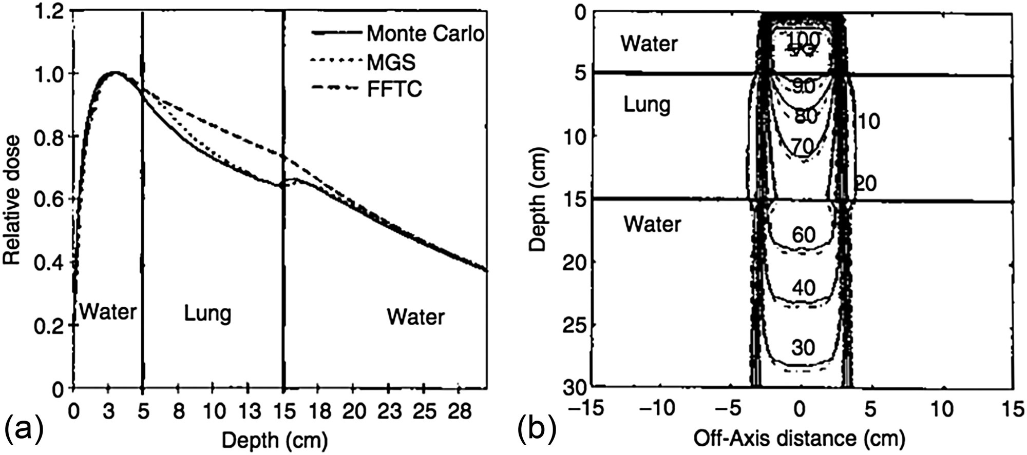
Bortfeld et al. (1993) stressed the inherent limitation: high accuracy is in principle only achievable for homogeneous phantoms with flat surfaces. Knöös et al. (1995) studied limitations in lung tissue in detail, comparing the Helax-TMS pencil beam model with Monte Carlo calculations in the challenging mediastinum geometry. Deviations in low-density volumes increased with beam energy: approximately 3% at 4 MV, reaching 14% at 18 MV — attributed to electron disequilibrium.
The conventional pencil beam is therefore classified as a type ‘a’ algorithm — it does not adequately account for secondary electron transport. Its use is not recommended for treatment planning in thoracic regions where electron disequilibrium is clinically significant. Details on these correction methods can be found in our article on empirical dose calculation methods.
Despite this limitation, the pencil beam remains available in many commercial systems as an acceptable speed-accuracy trade-off for most clinical situations, and it is particularly well suited for intensity modulation techniques including inverse planning.
Fast Pencil Beam: Speed for Real-Time Optimization
The Fast Pencil Beam is a simplified and accelerated variant of the convolutive pencil beam algorithm, designed specifically to provide real-time dose estimates during the iterative loops of IMRT and VMAT inverse optimization. While the conventional pencil beam already offers reasonable speed, the hundreds or thousands of iterations required in inverse planning demand an even faster calculation engine — and that is precisely the niche the Fast Pencil Beam fills.
How it works
The core strategy of the Fast Pencil Beam is to pre-compute lookup tables that store dose-per-unit-fluence values for each relevant combination of depth, lateral distance, and equivalent field size. During optimization, rather than executing the full convolution integral of Equation 28.32, the algorithm interpolates directly from these tabulated data. Scatter kernels are replaced by simplified models — often fixed-width Gaussians or low-order polynomials — that sacrifice lateral transport fidelity in exchange for a dramatic reduction in computation time.
Beyond lookup tables, typical implementations employ additional acceleration techniques: sparse sampling of the calculation grid (with interpolation at intermediate points), kernel truncation at lateral distances where the contribution is negligible, and representation of the modulated fluence at reduced resolution. The result is an algorithm capable of computing a complete dose distribution in fractions of a second — enabling the inverse optimizer to converge in minutes rather than hours.
Role in the clinical workflow
In clinical practice, the Fast Pencil Beam is not used as the final dose calculation algorithm. Its role is confined to the optimization engine: at each iteration of inverse planning, the optimizer evaluates hundreds of possible fluence configurations and requires a rapid response regarding the resulting dose. In this context, an estimate with 2–5% accuracy is sufficient to guide algorithm convergence.
Once the optimizer converges to an optimal fluence solution, the final dose calculation is performed with a higher-fidelity algorithm — typically AAA, Collapsed Cone Convolution (CCC), or in more modern systems, Monte Carlo or deterministic solvers such as Acuros XB. This two-stage approach — fast optimization followed by accurate final calculation — is the de facto standard in contemporary treatment planning systems.
Comparison with the conventional pencil beam
The differences between Fast Pencil Beam and the conventional pencil beam are not conceptual but rather implementational. Both are based on decomposing the beam into elementary pencils; the “fast” version, however, replaces physically detailed kernels with tabulated approximations. In homogeneous media, discrepancies between the two are generally below 2–3%. In heterogeneous media — particularly at lung-soft tissue interfaces and in build-up regions — the Fast Pencil Beam exhibits larger deviations than the conventional pencil beam, since the kernel simplifications further reduce the ability to model electron disequilibrium.
This accuracy loss is clinically acceptable during optimization because the goal at that stage is not to obtain the final dose, but rather to find the fluence map that best satisfies clinical constraints. The “real” dose is only evaluated after converting the optimized fluence into MLC segments and recalculating with the reference algorithm.
Commercial examples
The most prominent example is the Eclipse system (Varian), which uses the Fast Pencil Beam as its dose engine during IMRT and VMAT plan optimization, with final recalculation by AAA or Acuros XB. RayStation (RaySearch) employs a similar approach, with a fast pencil beam in the optimizer and CCC or Monte Carlo for the definitive calculation. In Pinnacle (Philips), CCC is used for both optimization and final calculation, which results in longer optimization times but dose consistency throughout the process.
The trend in newer systems is to replace the Fast Pencil Beam with GPU-based (Graphics Processing Unit) optimization engines, which allow more accurate algorithms — including accelerated CCC versions and even Monte Carlo — to run in times compatible with iterative optimization. Nevertheless, the Fast Pencil Beam remains in widespread clinical use and constitutes an essential step in the workflow of thousands of radiotherapy centers worldwide.
AAA in Eclipse: Beyond the Pencil Beam
The Analytical Anisotropic Algorithm (AAA) was implemented in Eclipse (Varian) in the early 2000s. It is essentially a pencil beam convolution/superposition algorithm with explicit, separate treatment of longitudinal and lateral components, scaled according to medium density.
The total dose is computed as the sum of contributions from beamlets $\beta$ covering the entire field area, each with a cross-section approximately matching the patient voxel size. For a water-like medium, the dose contribution at $P(x,y,z)$ from an individual beamlet $\beta$ at position $(x’,y’)$ is:
$$D_\beta(x,y,z) = I_\beta(z) \iint F_0(x’,y’) \, K_\beta(x-x’, y-y’, z) \, dx’ \, dy’ \quad (28.34)$$
Where $I_\beta(z)$ is the polyenergetic energy deposition function for primary photons at depth $z$, $F_0(x’,y’)$ is the incident primary fluence assumed uniform over the beamlet cross-section, and $K_\beta$ is the scatter kernel. The crucial difference from Equation 28.32: the primary energy deposition ($I_\beta$) is treated separately — not included in the scatter kernel.
The polyenergetic scatter kernel was represented in later versions (Tillikainen et al., 2007) as a sum of six radial exponential functions:
$$K_\beta(r,z) = \sum_{k=1}^{6} c_k \, \frac{1}{r} \, e^{-\mu_k r} \quad (28.35)$$
Where $r$ is the distance to the beamlet central axis, $\mu_k$ defines the range of scatter component $k$, and $c_k$ is the relative weight. In heterogeneous media, primary and scatter components are weighted by local relative density and scaled laterally using the water-equivalent path length. A recursive approach preserves the scaling “history” as depth increases.
AAA Performance and Limitations
Compared to the previous pencil beam in Eclipse, the AAA represented a significant improvement in dose calculation accuracy in heterogeneities. It can be considered a type ‘b’ algorithm — it approximately accounts for secondary electron transport (Knöös et al., 2006; Van Esch et al., 2006).
However, its electron transport treatment is not explicit — it uses lateral spread rather than the forward-directed spread of point kernels. This may cause apparent dose overestimation within and below low-density inhomogeneities for small fields in high-energy beams (Fogliata et al., 2007; Ding et al., 2006, 2007; Robinson, 2008; Dunn et al., 2015).
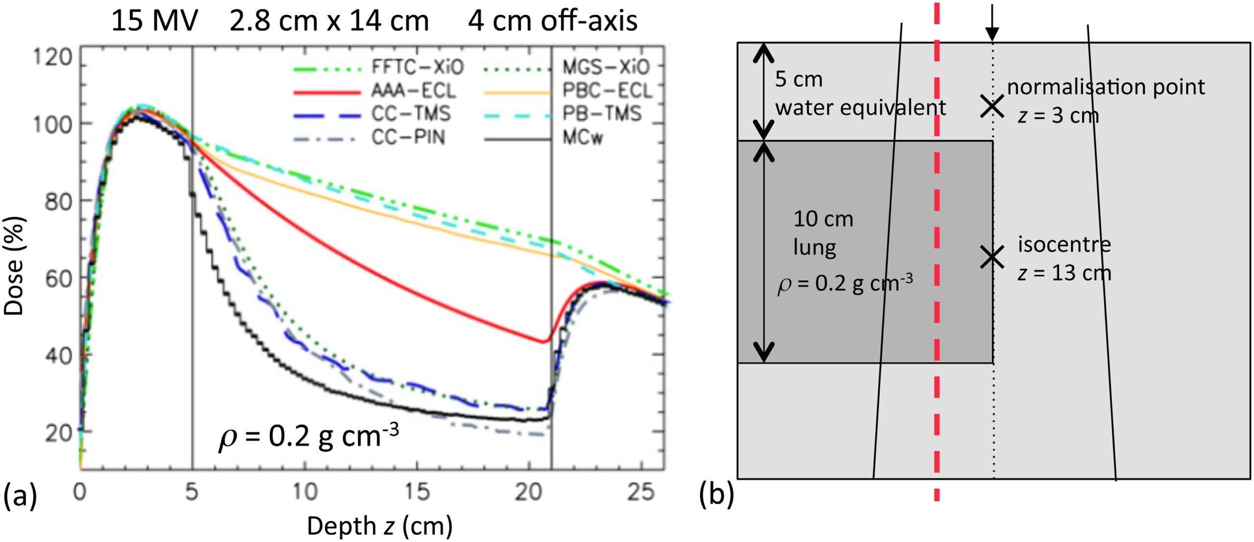
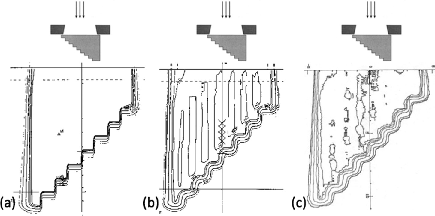
Figure 28.21 illustrates the issue clearly: for a 15 MV beam with a 2.8 cm × 14 cm field through 10 cm of lung-equivalent material ($\rho = 0.2$ g/cm³), type ‘a’ algorithms (FFTC-XiO, PB-TMS, PBC-ECL) fail to “see” the lack of electronic equilibrium. Type ‘b’ convolution/superposition algorithms (MGS-XiO, CC-TMS, CC-PIN) agree with Monte Carlo. The AAA (AAA-ECL) falls intermediate between these groups. For a comprehensive overview, see our complete guide on photon dose calculation algorithms.
Despite this limitation, the AAA is 4 to 10 times faster than a typical CCC point kernel algorithm (Hasenbalg et al., 2007; Han et al., 2011). For cases where it is less accurate, the alternative on the Eclipse platform is the model-based Acuros XB algorithm.
Electron Pencil Beam: The Fermi–Eyges Model
The pencil beam concept also applies to charged particles, but the underlying physics changes radically. Unlike photons, electrons interact “immediately” and “continuously” upon entering the medium. The Hogstrom model (1981), based on Fermi–Eyges theory, dominated electron dose calculation since the early 1980s. The analytical solution provides the probability of finding an electron at depth $z$ with lateral displacement $(x,y)$:
$$p(x,y,z) \, dx \, dy = \frac{1}{2\pi \sigma_{MCS}^2} \exp\left(-\frac{x^2 + y^2}{2\sigma_{MCS}^2}\right) dx \, dy \quad (29.1)$$
Where $\sigma_{MCS}^2 = \frac{1}{2} \int_0^z (z-u)^2 T(u) du$ is the accumulated multiple Coulomb scattering, and $T(u)$ is the linear scattering power of the medium at depth $u$.
Critical limitations
The most serious limitation is the central-ray approximation: each pencil is corrected for inhomogeneities based only on material along its central ray, equivalent to assuming a layered phantom. Additionally, Fermi–Eyges theory predicts continuously increasing $\sigma_{MCS}(z)$ with depth, while the true behavior shows a maximum followed by decrease due to range straggling. These limitations drove the development of Monte Carlo methods for electron dose calculation.
Proton Pencil Beams
High-energy proton beams follow analogous principles. The simplest approach, ray tracing, only accounts for range changes without predicting lateral effects. The pencil beam substantially improves modeling by including lateral scatter, capturing the Bragg peak “degradation” caused by heterogeneous structures — producing smoother, more realistic isodoses that better match measurements.
Comparisons between Eclipse, XiO and Pinnacle for meningioma cases (Doolan et al., 2015) demonstrate clinically relevant differences between algorithms, especially at bone-soft tissue interfaces.
Commercial Algorithm Comparison
| Feature | Pencil Beam | Fast Pencil Beam | AAA | CCC | Monte Carlo |
|---|---|---|---|---|---|
| Classification | Type ‘a’ | Type ‘a’ (simplified) | Type ‘b’ (intermediate) | Type ‘b’ | Reference |
| Secondary e⁻ transport | Not explicit | Not explicit | Approximate (lateral spread) | Yes (via kernels) | Yes (explicit) |
| Heterogeneities | Depth scaling | Simplified scaling | Anisotropic scaling (recursive) | 3D density scaling | Full transport |
| Lung error (18 MV) | Up to 14% | >14% (critical heterogeneities) | Intermediate (~5-8%) | ~2-3% | <1% (reference) |
| Relative speed | Very fast (FFT) | Ultra-fast (lookup tables) | Fast | 4-10× slower than AAA | Very slow |
| Primary use | Final calculation in simple cases | Inverse optimization engine | Final calculation (Eclipse) | Final calculation (Pinnacle, XiO) | Reference / final calculation |
| Commercial TPS | Eclipse, Helax-TMS | Eclipse (IMRT/VMAT optimizer) | Eclipse (Varian) | Pinnacle, XiO, TMS | Monaco, iPlan |
Source: Compiled from the Handbook of Radiotherapy Physics, 2nd Ed. (CRC Press, 2020)
Algorithm selection depends on the clinical scenario. For routine planning without major heterogeneities, pencil beam or AAA provide adequate accuracy with superior speed. The Fast Pencil Beam plays a fundamental behind-the-scenes role in inverse optimization, but should never be used as the final dose calculation. For thoracic regions with small fields and high-energy beams, type ‘b’ algorithms like CCC — or ideally model-based solutions such as Acuros XB or Monte Carlo — are strongly recommended.
For a complete overview of the entire dose calculation algorithm journey — from empirical methods through Monte Carlo and Acuros — see our complete guide on photon dose calculation algorithms.