
Monte Carlo Patient Dose Calculation
Patient dose calculation is the ultimate goal of any Monte Carlo (MC) simulation in radiation therapy. Unlike simplified analytical models, MC tracks every single particle — and that changes everything. The major codes available today are EGSnrc, MCNP, GEANT4, and PENELOPE, all built on the condensed history technique first proposed by Berger in 1963, where thousands of electron interactions are grouped into macroscopic steps.
Two implementation classes exist. In class I (used by MCNP/ETRAN), all collisions are grouped, and secondary particles above an energy threshold are created after the fact. In class II (EGSnrc, GEANT4, PENELOPE), “hard” or catastrophic collisions are tracked individually while “soft” collisions follow the class I scheme. Step-size artifacts and boundary-crossing issues are now well understood and resolved — significantly improving the accuracy of modern MC codes. For a comprehensive overview, see our complete guide to Monte Carlo in Radiotherapy.
In This Article
Statistical Uncertainties and Scoring Geometries
Every MC simulation introduces unavoidable statistical noise in the calculated dose. The fluctuation around the mean value in each voxel — characterized by the variance $\sigma^2$ — directly affects isodose lines and dose-volume histograms (DVHs). In an ideal simulation, zero variance would be the goal, but that requires infinite computation time.
MC calculation performance is measured by efficiency $\varepsilon$, defined as:
$$\varepsilon = \frac{1}{\sigma^2 T}$$
Where:
- $\sigma^2$ = estimate of the true variance on the quantity of interest
- $T$ = CPU time required to achieve that variance
To improve efficiency, we can either reduce $\sigma^2$ for a given $T$ (variance reduction techniques) or reduce $T$ for a given $N$ without changing the variance.
Scoring Geometries: Dosels, Kugels, and Segmented Organs
Not all scoring needs to happen on regular cubic voxels. The PEREGRINE dose engine, for example, uses dosels — overlapping spheres independent of the material transport mesh. The simulation monitors the standard deviation in the highest-dose dosel and terminates when it reaches the user-specified level.
Another approach uses kugels, employed by the Macro Monte Carlo (MMC) engine. Electrons are transported in macroscopic steps through spheres of various materials and radii, with pre-calculated results stored in lookup tables. The concept, introduced by Neuenschwander et al. (1995), enables fast treatment planning calculations for electron beams.
When individual voxels are combined into larger volumes — such as segmented organs — spatial resolution is lost, but speed and accuracy in organ dose prediction improve significantly. The limitation? Volume contouring depends heavily on the clinician performing it. That is why organ-based scoring works best in controlled environments like the NCAT phantom, based on the Visible Human dataset, which models 3D anatomy with NURBS surfaces and incorporates 4D respiratory and cardiac motion.
Voxel Size Effects and Latent Variance
Scoring voxel size directly impacts calculation time, as it determines the time spent on boundary-crossing checks. Cygler et al. (2004) showed that the number of histories required per unit area is linearly proportional to the scoring voxel mass.
There is also latent variance, a concept coined by Sempau et al. (2001). This is the residual uncertainty arising from statistical fluctuations in the phase space generated by the treatment head simulation. Even reusing phase space particles infinitely many times, the uncertainty converges to this finite, irreducible value. If latent variance is significant in the total uncertainty budget, more independent phase space particles must be generated.
Uncertainty Estimation Methods
The batch method divides histories into $N$ batches (typically 10) and estimates uncertainty as:
$$s_{\bar{X}} = \sqrt{\frac{\sum_{i=1}^{N}(X_i – \bar{X})^2}{N(N-1)}}$$
Walters et al. (2002) identified three problems: (1) few batches cause fluctuations in the uncertainty itself, (2) arbitrary grouping ignores particle correlations, and (3) the method adds an extra dimension to scored quantities.
The history-by-history method, implemented following Salvat’s approach, solves these problems by maintaining running sums of $\sum X_i^2$ and $\sum X_i$ during the simulation, computing the final uncertainty via:
$$s_{\bar{X}} = \sqrt{\frac{1}{N(N-1)} \left[ \sum_{i=1}^{N} X_i^2 – \frac{\left(\sum_{i=1}^{N} X_i\right)^2}{N} \right]}$$
This eliminates the need to store batch data and is computationally more efficient.
Denoising and Smoothing Methods
Reducing statistical fluctuations by simulating more histories is the pure approach, but impractical without powerful variance reduction techniques. The alternative is removing noise a posteriori with denoising algorithms — analogous to image restoration — to speed up MC calculations.
Kawrakow (2002) established five accuracy criteria that became the standard for evaluating smoothing algorithms:
- Visual inspection of isodose lines (minimal differences from benchmark)
- Area difference between smoothed and reference DVHs
- Maximum dose difference
- RMSD (root-mean-square difference) between distributions
- x%/y mm test — fraction of voxels differing by more than x% with no benchmark point closer than y mm (current recommendation: 2-3%/2 mm)
DVH Denoising
Sempau and Bielajew (2000) proposed treating the calculated DVH as a convolution of the true DVH (zero variance) with noise, applying deconvolution to recover the original signal. In practice, DVH-based decisions could be made quickly, enabling MC use throughout the inverse planning process.
Jiang et al. (2000) adopted a similar approach, treating the MC DVH as a blurred image and applying iterative least-squares minimization to restore it.
3D Dose Distribution Denoising
DVH denoising does not fully address the problem since dose distributions are evaluated in multiple ways (isodoses, TCP/NTCP). Several methods target the 3D distribution directly:
Digital filtering (Deasy, 2000) — First to propose 3D denoising, demonstrated that digital filters improve visual usability and clinical reliability of MC dose distributions for electrons.
Wavelets (Deasy et al., 2002) — Wavelet coefficients below a threshold are set to zero, suppressing noise with minimal bias introduction. Speedup of 2x or more.
3D Savitzky-Golay (Kawrakow, 2002) — 3D generalization with adaptive window size based on local uncertainty. Reduces required histories by factors of 2 to 20. Extremely useful in the iterative trial-and-error phase of treatment planning.
Adaptive anisotropic diffusion (Miao et al., 2003) — Filtering parameters are modified according to local noise. Reduces noise 2-5x (up to 20x in simulation time) while preserving dose gradients.
IRON (Fippel and Nusslin, 2003) — Iterative noise reduction algorithm minimizing second partial derivatives of dose. Speedup of 2 to 10x in calculation time.
Content adaptive median hybrid filter (El Naqa et al., 2005) — Combines median operator in strong gradient regions with mean operator in homogeneous regions, merging outlier removal with smoothness.
| Method | Author(s) | Speedup Factor | Key Feature |
|---|---|---|---|
| Digital filtering | Deasy (2000) | — | Pioneer in 3D denoising for MC electron beams |
| Wavelets | Deasy et al. (2002) | 2x | Wavelet coefficient thresholding |
| 3D Savitzky-Golay | Kawrakow (2002) | 2-20x | Adaptive window by local uncertainty |
| Anisotropic diffusion | Miao et al. (2003) | up to 20x | Preserves dose gradients |
| IRON | Fippel and Nusslin (2003) | 2-10x | Iterative second-derivative minimization |
| Median-mean hybrid | El Naqa et al. (2005) | — | Adaptive by gradient region |
Source: Monte Carlo Techniques in Radiation Therapy (2nd ed., CRC Press, 2022), Chapter 11
CT to Medium Conversion: Stoichiometric Methods
Converting CT Hounsfield units (HU) into material composition and mass density is one of the most critical links for MC dose calculation accuracy. Getting this wrong compromises everything downstream.
Early algorithms used only 6 materials (air, lung, fat, water, muscle, bone). du Plessis et al. (1998) investigated the influence of tissue composition and concluded that 7 basic tissue subsets were sufficient for 1% dose accuracy with megavoltage photon beams. They constructed 57 tissue types by varying physical density for lung and cortical bone, spanning 3,000 HU.
Schneider Stoichiometric Conversion
The stoichiometric conversion, proposed by Schneider et al. (1996) initially for protons, was a major step forward. Materials of known composition are CT-scanned to measure corresponding HU values. Measured values are fitted using Rutherford et al.’s (1976) parameterization:
$$\sigma_i(E) = Z_i \left[ K_{KN}(E) + Z_i^{1.86} K_{sca}(E) + Z_i^{3.62} K_{ph}(E) \right]$$
Where $K_{KN}$ is the Klein-Nishina coefficient, $K_{sca}$ the Rayleigh scattering coefficient, and $K_{ph}$ the photoelectric coefficient. The linear attenuation coefficient $\mu$ is obtained via:
$$\mu(E) = \rho \frac{N_A}{A} \sum_{i=1}^{n} \frac{w_i}{A_i} \sigma_i(E)$$
Schneider et al. (2000) expanded the method to 71 human tissues, creating 4 sections on the CT scale where density and elemental weights are interpolated between two reference tissues. The composite tissue density is:
$$\rho = \frac{\rho_1 \rho_2}{W_1(\rho_2 – \rho_1) + \rho_1}$$
Where $W_1$ and $W_2 = 1 – W_1$ represent the proportions of the two reference tissues.
Dosimetrically Equivalent Subsets (14 bins)
Vanderstraeten et al. (2007) generalized the method, creating 14 dosimetrically equivalent tissue subsets (10 of which were bone), ensuring tissues at the interface between two bins did not differ by more than 1% in dose. Comparison with the conventional 5-bin scheme showed differences up to 5% at interfaces — particularly between adipose tissue and bone. While DVHs showed no significant differences, point-dose accuracy improved substantially.
Dual-Energy CT for Improved Conversion
Dual-energy CT scans with two significantly different tube voltages to better estimate effective atomic numbers $Z$ and relative electron densities $\rho’_e$. Bazalova et al. (2008) found mean extraction errors of $\rho’_e$ and $Z$ of 1.8% and 2.8%, respectively.
| Beam Energy | Type | Dose Error from Misassignment |
|---|---|---|
| 250 kVp | X-rays | 17% |
| 6 MV | Photons | < 1% |
| 18 MV | Photons | 3% |
| 18 MeV | Electrons | 6% |
Source: Monte Carlo Techniques in Radiation Therapy (2nd ed., CRC Press, 2022), Chapter 11
In practice, dual-energy CT provides the greatest advantage for low-energy beams where $Z$-dependence is strongest.
Deformable Image Registration and 4D Dose
Respiratory motion in lung radiotherapy poses a real challenge for dosimetric accuracy. Deformable image registration (DIR) enables mapping dose distributions between breathing phases, making 4D MC dose calculation feasible.
Keall et al. (2004) performed one of the first pseudo-4D MC calculations: dose computed on each of $N=8$ individual 3D CT cubes representing breathing phases, then mapped back to the reference phase via DIR. Multiple algorithms exist — accelerated Demons, B-splines respecting pleural discontinuity, optical flow, thin-plate spline, and finite element methods. For more on dynamic beam delivery and 4D simulations, see our article on Dynamic Beam Delivery and 4D Monte Carlo.
Dose Warping Approaches
Heath and Seuntjens (2006) developed defDOSXYZnrc, which warps the dose grid on the fly while tracking individual particles. The disadvantage: calculation time increases by a factor of 2 or more.
Siebers and Zhong (2008) proposed the Energy Transfer Method (ETM), separating radiation transport from energy deposition. When two voxels $A_1$ and $A_2$ merge into $X_1$ after registration, simple interpolation calculates:
$$d_{INTERP}(X_1) = \frac{d(A_1) + d(A_2)}{2}$$
But the correct interpretation considers energy transfer:
$$d_{ETM}(X_1) = \frac{E(A_1) + E(A_2)}{m(A_1) + m(A_2)}$$
This correction is especially important in dose gradient regions, where energy per unit mass redistributes non-linearly.
3D vs. 4D: How Much Does Motion Matter?
Flampouri et al. (2005) studied six lung IMRT patients and concluded that conventional planning was sufficient for tumors with motion less than 12 mm. For larger motion or severe CT artifacts, 4D MC becomes necessary. Striking finding: CT reconstruction artifacts have a bigger effect than tumor motion itself.
Seco et al. (2008) compared 3D FB with 4D FB and 4D gated treatments, introducing the omega index $\Omega(\rho)$ to analyze dose differences as a function of tissue density:
$$\Omega(\rho) = \frac{\int f(\mathbf{x}) \, \delta(\rho(\mathbf{x}) – \rho) \, d\mathbf{x}}{\int \delta(\rho(\mathbf{x}) – \rho) \, d\mathbf{x}}$$
Differences of 3-5 Gy between inhalation and free-breathing were observed in both low-density (lung) and high-density (bone) regions. 4D MC improves predictions not only within the tumor but also in surrounding tissues that make up the expanded PTV. No significant dosimetric differences were observed between 4D FB and 4D gated in the three patients evaluated.
In the dose warping intercomparison by Heath et al. (2008), the three tested methods (center of mass tracking, trilinear interpolation, and defDOSXYZ) showed no clinically significant dose differences. However, when motion was not accounted for, target volume dose was underestimated by up to 16%.
Inverse Planning with Monte Carlo
In IMRT planning, the $D_{ij}$ matrix converts fluences into dose distribution:
$$D(x_i) = \sum_{j \in \text{Beamlet}} D_{ij} \, x_j$$
Where $D_{ij}$ is the dose influence and $x_j$ is each beamlet intensity. This matrix can be calculated using pencil beam (PB), superposition-convolution, or MC algorithms. The problem: MLC delivery constraints and field-size-dependent output factor dependencies are usually not accounted for in $D_{ij}$ generation, leading to suboptimal delivered dose distributions.
Jeraj and Keall (1999) pioneered MC inverse planning using MCNP for initial fluence generation and EGS4 for patient dose calculation. The limitation: MC pencil beams did not model the actual linac spectrum, MLC constraints, or head scatter variations.
Siebers and Kawrakow (2007) proposed a hybrid method where the initial prediction uses PB and subsequent iterations correct with MC, achieving a 2.5x gain over full MC-based optimization.
Broad Beam Approach (Nohadani et al., 2009)
Nohadani et al. used an open-field phase space after the jaws (which do not change during IMRT delivery on Varian linacs) split into PB-like pixels. Three clear advantages: (1) accounts for patient heterogeneities, (2) the output factor is that of standard open field with no additional corrections, and (3) output variations from field size changes during MLC delivery are small and do not affect the optimized plan.
Comparing DVHs of IMRT plans optimized with MC-PB versus conventional PB revealed something important: the PB-based plan appears better in terms of PTV coverage, hot spots, and organ-at-risk sparing — but it deviates significantly from the actual deposited dose. Dose calculation errors cannot be neglected in clinical planning.
Clinical Applications for Electron Beams
For electron beams, MC demonstrates clear advantages over analytical algorithms like pencil beam. In heterogeneities (bone, air, lung), pencil beam fails to predict lateral scattering, backscatter, and cavity effects — situations where MC excels by tracking each particle through all relevant physical interactions, including explicit modeling of the machine and patient geometry.
Commissioning an MC-based TPS for electrons requires attention to: calculation verification against measured data, dose normalization and prescription, statistical uncertainty versus voxel size, and the distinction between dose-to-medium and dose-to-water. Learn more about Monte Carlo for electrons and brachytherapy in our dedicated article.
The evolution of commercial MC TPSs for electrons brought clinically acceptable calculation times — around 4 minutes for calculations with 2% statistical uncertainty and 0.25 cm voxel size. Initiatives like the OMEGA project and EGSnrc-based implementations paved the way for commercial packages used in clinical routine today.
Final Considerations
Monte Carlo patient dose calculation has evolved from an academic tool to a viable component of clinical planning systems. Advances in denoising (2-20x calculation time reductions), stoichiometric CT conversion (from 5 bins to 14 dosimetrically equivalent bins), and MC inverse planning enable more accurate calculations without sacrificing practicality.
For electron applications, where tissue heterogeneities challenge conventional algorithms, MC offers the definitive solution — provided it is accompanied by rigorous commissioning. With the growing integration of 4D deformable registration, MC is moving toward capturing not just static anatomy but the full respiratory dynamics of the patient.
To dive deeper into Monte Carlo fundamentals or explore how the method applies to photons in clinical applications, check out our dedicated articles in this series.
Main source: Monte Carlo Techniques in Radiation Therapy (2nd ed., CRC Press, 2022), Chapters 11-12.