Monte Carlo is no longer confined to research centres. Treatment planning systems such as Monaco (Elekta), iPlan (BrainLab), and options within Eclipse (Varian) now offer stochastic dose calculation — while the deterministic Acuros XB engine delivers comparable accuracy in a fraction of the time. This article explores how Monte Carlo works in the clinical setting, which MC codes underpin commercial TPS platforms, and why the Boltzmann transport equation solved by Acuros XB is reshaping the medical physicist’s daily workflow.
For a comprehensive overview of dose calculation evolution — from empirical methods to convolution techniques — see our complete guide on photon dose calculation algorithms.
Monte Carlo in Radiotherapy: Why Simulate Particle by Particle?
Monte Carlo numerically solves the Boltzmann transport equation by tracking millions of individual particles. Unlike analytical algorithms that approximate transport with kernels or pencil beams, MC reproduces every photon–electron interaction according to known cross-sections. The result is the most accurate dose distribution computationally achievable.
The simulation starts from the phase-space — energy, position, and direction of each particle. A 1 MeV photon undergoes on average 14–15 interactions in water before photoelectric absorption. Each interaction is selected by random sampling from the cumulative probability distribution (CPD): pair production, Compton scattering, photoelectric absorption, and Rayleigh scattering. The distance to the next interaction follows:
$$x = -\frac{1}{\mu_{tot}} \ln(1 – R)$$
Where:
- $\mu_{tot}$ = total attenuation coefficient of the medium (sum of all interaction processes)
- $R$ = uniformly distributed random number between 0 and 1
For electrons, the picture changes dramatically. A 10 MeV electron in oxygen has a CSDA range of 5.6 g/cm² and undergoes between $10^5$ and $10^6$ interactions before losing all kinetic energy. Simulating each one individually would be computationally prohibitive.
Condensed History Electron Transport
The solution came from Berger (1963): the condensed history method. The idea is to group thousands of small-effect interactions into a manageable number of virtual large-effect steps. Between so-called “catastrophic” collisions — delta-ray creation and bremsstrahlung photon generation above certain thresholds — the electron loses energy continuously according to the restricted stopping power.
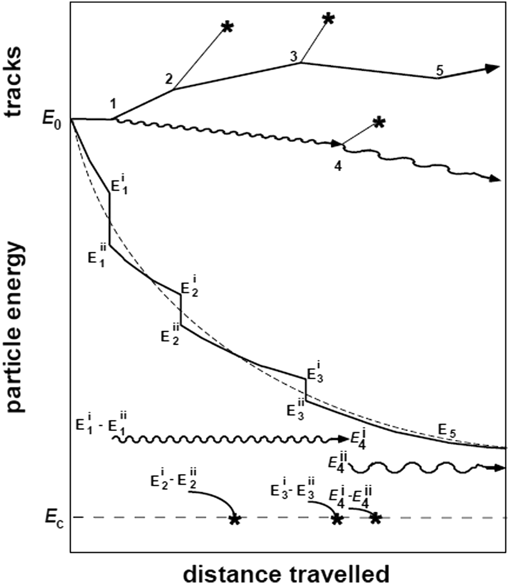
Berger classified this approach as “Class II” simulation: a hybrid between continuous transport and analogue sampling of discrete events. Energy cutoffs control the trade-off between accuracy and speed. In EGSnrc, the ECUT parameter defines the kinetic energy below which the electron is “absorbed locally” — typically chosen so the CSDA range at that energy is about 1/3 of the smallest voxel dimension. The ESTEPE parameter limits the maximum fractional energy loss per condensed step (typical value: 4%).
Without condensed history, charged particle transport would require teraflop-scale ($10^{12}$ operations/second) resources for most practical problems. In practice, condensed history is the single most important variance reduction technique in radiotherapy applications.
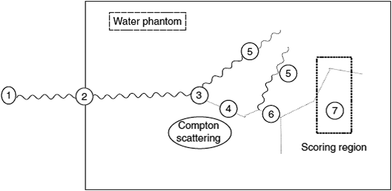
Coupled Photon–Electron Transport
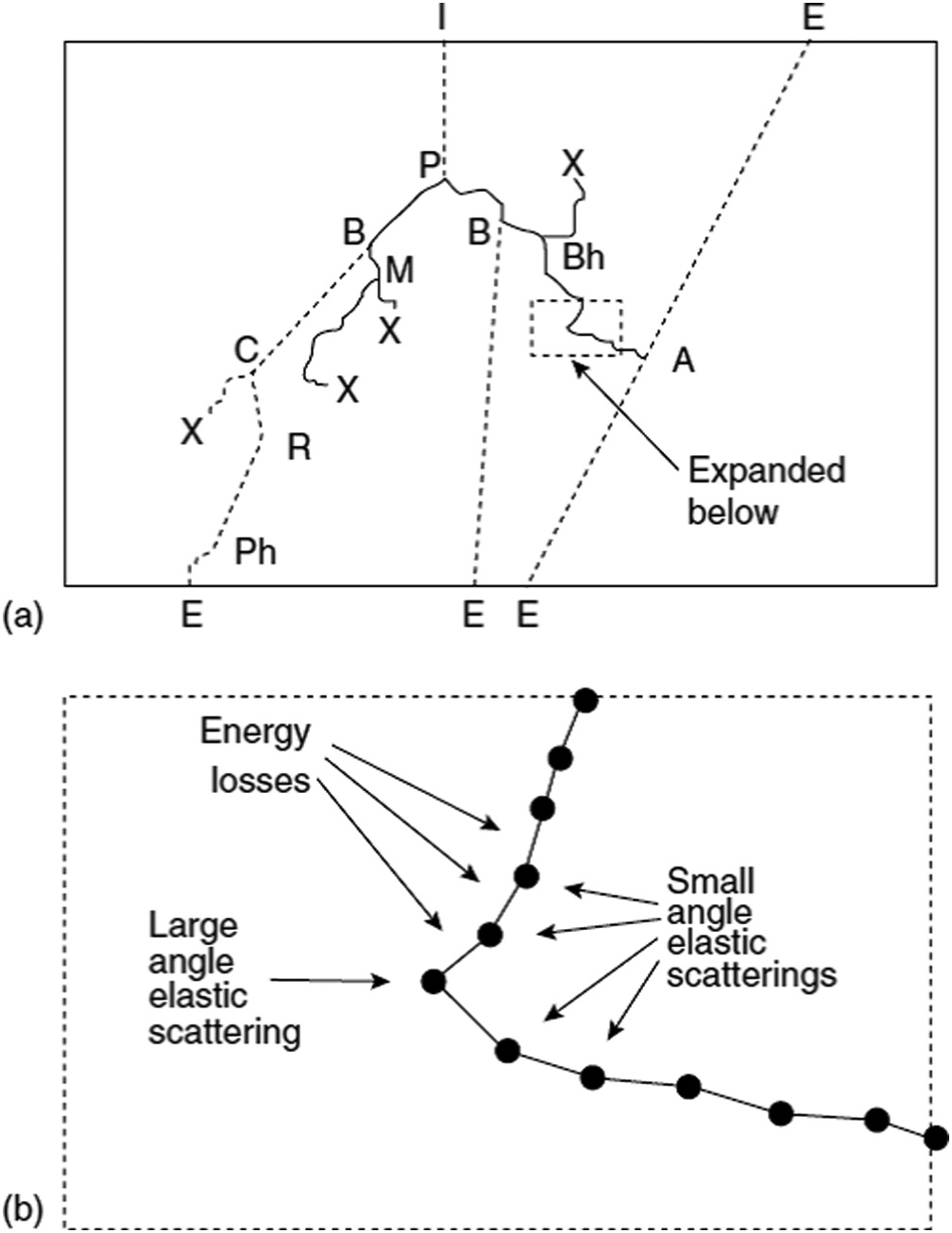
Photons transfer energy through secondary electrons — so transport of both particle types must be coupled. Figure 30.5 illustrates a complete history: a photon enters the geometry and undergoes pair production (P). The resulting electron generates bremsstrahlung (B), while the scattered photon undergoes Compton (C), Rayleigh (R), and photoelectric absorption (Ph). The positron annihilates (A) producing two 511 keV photons that escape the geometry.
In clinical practice, this coupling allows Monte Carlo to correctly capture effects such as charged particle disequilibrium in small fields and density interfaces — situations where algorithms like pencil beam and AAA can fail significantly.
Variance Reduction Techniques in Monte Carlo
The statistical uncertainty of an MC simulation decreases with $1/\sqrt{N}$, where $N$ is the number of histories. Doubling precision requires quadrupling computation time. Variance reduction techniques (VRTs) overcome this bottleneck by modifying the simulation to achieve lower variance without increasing the number of histories.
The efficiency $\varepsilon$ of a simulation is defined as:
$$\varepsilon = \frac{1}{[s(N)]^2 \cdot T(N)}$$
Where $[s(N)]^2$ is the estimated variance and $T(N)$ the total computation time. The goal of VRTs is to increase $\varepsilon$ by reducing $s(N)$, $T(N)$, or both.
The most widely used VRTs in linac head simulation include:
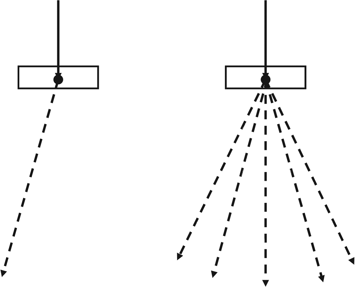
- Uniform particle splitting: instead of generating 1 bremsstrahlung photon with weight $w = 1$, $N_{split}$ independent photons are created with weight $w = 1/N_{split}$ each. Figure 30.7 shows the concept with $N_{split} = 5$.
- Interaction forcing: photons are forced to interact within the region of interest. The number of mean free paths $\lambda$ to the interaction point is: $\lambda = -\ln\left[1 – R(1 – e^{-\Lambda})\right]$, where $\Lambda = \sum_{Start}^{Stop} \mu_i s_i$.
- Correlated sampling: transport in the outer (constant) region is pre-computed, and only transport in the variable region is repeated for each different geometry.
- Russian roulette: eliminates low-weight particles, compensating with a proportional increase in survivors’ weights.
MC Codes and Commercial TPS Implementations
The modern medical physicist no longer needs to write MC code from scratch. Decades of development have produced powerful packages, many freely available. The table below summarises the main codes used in medical physics.
Major Monte Carlo Codes in Medical Physics
| Code | Key Features | Application |
|---|---|---|
| EGSnrc / BEAMnrc | Most cited code in medical physics; fine control of condensed history electron–photon transport | Research; linac head modelling (BEAMnrc); patient dose (DOSXYZnrc) |
| MCNP | Includes neutron transport; extensive use in nuclear industry | Medical physics; shielding; brachytherapy |
| GEANT4 | Comprehensive multi-particle toolkit; growing medical use | Research; proton therapy; PET/SPECT |
| VMC++ / XVMC | Optimised for speed with “electron-track repeating” | Oncentra/Masterplan (Elekta); Monaco; XiO |
| PENELOPE | Sophisticated electron transport algorithms | Research; PRIMO (free verification) |
| DPM | Large condensed history steps crossing material interfaces | Pinnacle TPS (Philips) |
| MMC (Macro MC) | Semi-numerical, fast hybrid electron transport | Eclipse (Varian) — electron beams |
| PEREGRINE | Built specifically for radiotherapy planning | Corvus (Best NOMOS) |
Source: Handbook of Radiotherapy Physics: Theory and Practice, 2nd Ed. (CRC Press, 2020) (Table 30.1)
Commercial TPS with Monte Carlo
| TPS / System | Type | Linac Simulation | Patient Dose | Availability |
|---|---|---|---|---|
| Monaco (Elekta) | Planning | VSM | XVMC (fast) | Commercial |
| Eclipse — electrons (Varian) | Planning | VSM | MMC (pre-calculated) | Commercial |
| iPlan (BrainLab) | Planning | VSM | XVMC (fast) | Commercial |
| Oncentra (Elekta) | Planning | VSM | VMC++ (fast) | Commercial |
| Pinnacle (Philips) | Planning | — | DPM (fast) | Commercial |
| XiO (Elekta) | Planning | VSM | XVMC (fast) | Commercial |
| PRIMO | Verification | PENELOPE (full) | PENELOPE | Free |
| PLanUNC | Verification | EGSnrc (full) | EGSnrc | Free |
Source: Handbook of Radiotherapy Physics: Theory and Practice, 2nd Ed. (CRC Press, 2020) (Table 30.2, adapted)
Clinical Monte Carlo: Dose per MU and Dose-to-Medium
Two practical issues distinguish clinical MC from research MC. First is the dose per monitor unit (MU) relationship. MC calculates dose per simulated particle — to convert to Gy/MU, normalisation against the dose under reference conditions (10×10 cm² field, reference depth, defined SSD or SAD) is required. This calibration ensures consistency with the service’s absolute dosimetry.
The second issue is the choice between dose-to-medium ($D_m$) and dose-to-water ($D_w$). MC naturally computes $D_m$ — the dose deposited in the actual voxel material (bone, lung, soft tissue). To convert to $D_w$, the water/medium stopping power ratio is applied:
$$D_w = D_m \cdot \left(\frac{S}{\rho}\right)_{medium}^{water}$$
In practice, the difference between $D_w$ and $D_m$ is clinically significant only in bone (up to 5–10%) and may influence DVH interpretation in head-and-neck or spine cases.
Why Hasn’t MC Taken Over Clinical Routine?
Unprecedented accuracy comes at a price: computation time. Around 1990, a photon treatment plan was estimated to require hundreds of hours with available hardware. Today, with multicore processors and GPUs, clinical MC is feasible for electron beams and approaching full feasibility for photons.
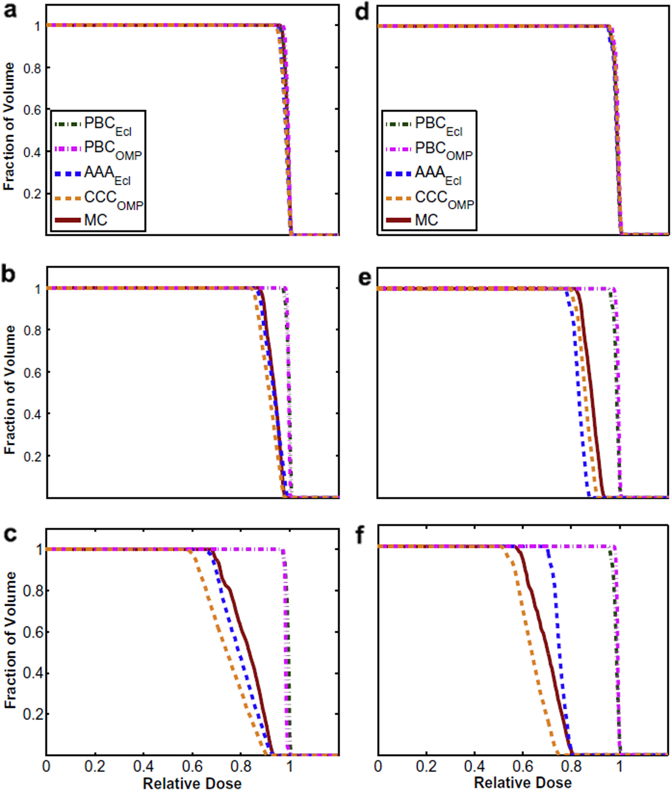
Figure 30.13 shows DVHs for a lung tumour computed with different algorithms. At lung density 1.0 g/cm³, all methods agree. As density drops to 0.4 and then 0.1 g/cm³, pencil beam algorithms severely overestimate tumour dose, while MC and Collapsed Cone Convolution converge. At 18 MV and 0.1 g/cm³ density, the pencil beam discrepancy exceeds 20%.
The fundamental reason for this superiority is shown in Figure 30.12: rectilinear kernel scaling (used by convolution algorithms) assumes dose distribution depends only on the average density between interaction and deposition points. MC shows that the order of densities matters — a photon crossing dense tissue first and then lung produces a different electron pattern than the reverse path. To learn more about superposition and TERMA fundamentals, see our dedicated article.
The Linear Boltzmann Transport Equation (LBTE): Mathematical Foundations
While Monte Carlo solves the transport equation stochastically — simulating individual particle histories — Acuros XB takes the deterministic approach: solving the LBTE directly on a computational grid. To understand Acuros, one must first understand the equation it solves.
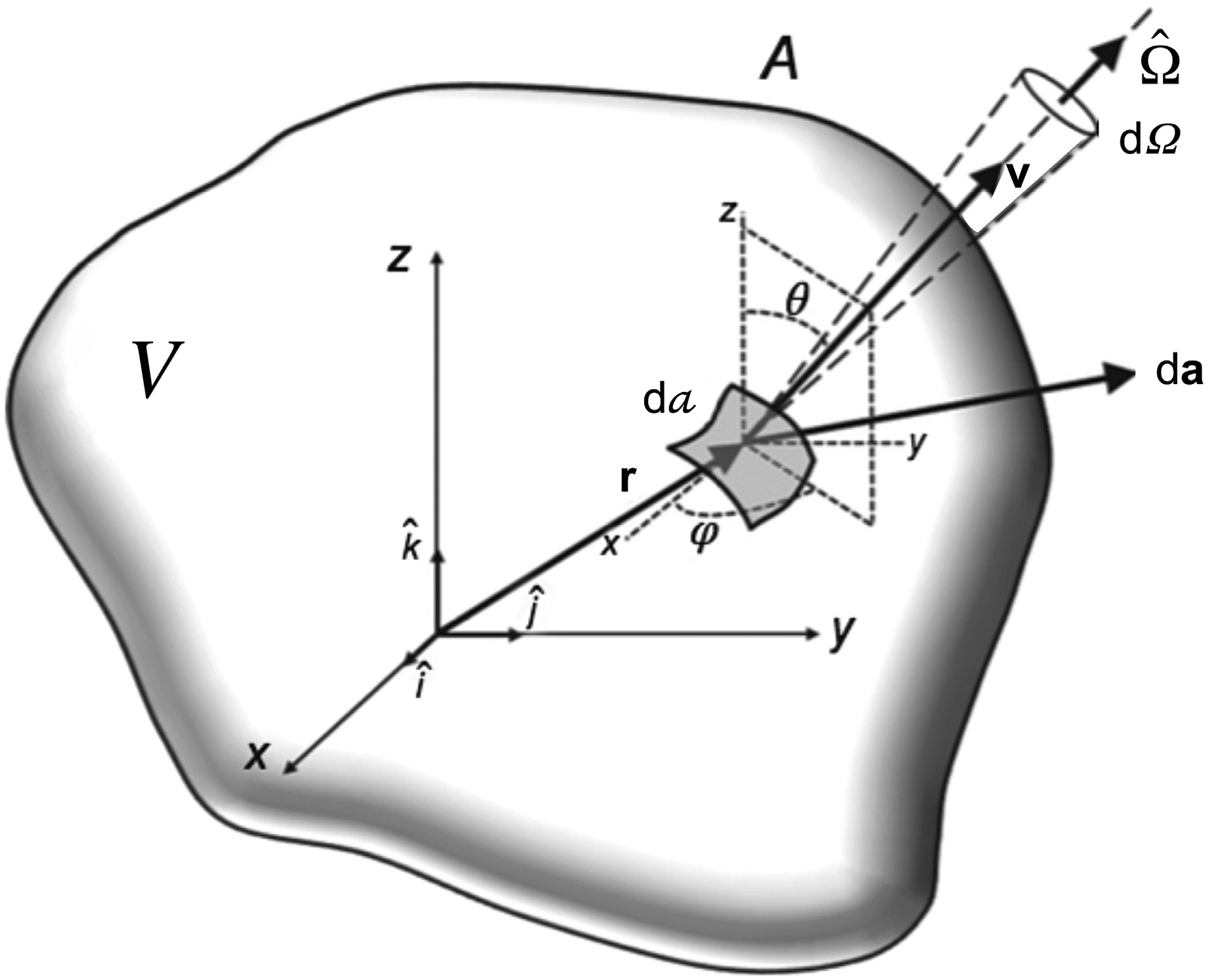
The linear Boltzmann transport equation describes particle conservation in a medium. In its most general form, for a particle of type $p$ with energy $E$ travelling in direction $\hat{\Omega}$ from position $\vec{r}$:
$$\hat{\Omega} \cdot \nabla \psi_p(\vec{r}, E, \hat{\Omega}) + \sigma_{t,p}(\vec{r}, E)\, \psi_p(\vec{r}, E, \hat{\Omega}) = q_p(\vec{r}, E, \hat{\Omega})$$
Where:
- $\psi_p(\vec{r}, E, \hat{\Omega})$ = angular fluence of particle type $p$ (photons or electrons) at position $\vec{r}$, energy $E$ and direction $\hat{\Omega}$
- $\sigma_{t,p}(\vec{r}, E)$ = total macroscopic cross-section (interaction probability per unit path length)
- $q_p(\vec{r}, E, \hat{\Omega})$ = total source term, including scattering-in, secondary particle production, and external sources
- $\hat{\Omega} \cdot \nabla$ = streaming operator (spatial derivative along the flight direction)
The first term ($\hat{\Omega} \cdot \nabla \psi$) describes free particle transport along direction $\hat{\Omega}$. The second term ($\sigma_t \psi$) represents losses due to interactions — both absorption and out-scattering from the angular beam considered. The right-hand side ($q_p$) groups all particle sources at that point in phase space.
The source term is the most complex part of the equation, as it couples different particle types and energies:
$$q_p(\vec{r}, E, \hat{\Omega}) = \sum_{p’} \int_0^{\infty} \int_{4\pi} \sigma_{s,p’ \to p}(\vec{r}, E’ \to E, \hat{\Omega}’ \to \hat{\Omega})\, \psi_{p’}(\vec{r}, E’, \hat{\Omega}’)\, d\hat{\Omega}’\, dE’ + q_{ext,p}(\vec{r}, E, \hat{\Omega})$$
Here, $\sigma_{s,p’ \to p}$ is the differential scattering kernel describing the probability of a particle of type $p’$ with energy $E’$ and direction $\hat{\Omega}’$ producing a particle of type $p$ with energy $E$ and direction $\hat{\Omega}$. The summation over $p’$ couples photons and electrons: Compton photons generate electrons, electrons generate bremsstrahlung, and so on.
Coupled Photon–Electron Transport in the LBTE
For clinical megavoltage beams, the LBTE unfolds into a coupled system. Photon transport follows:
$$\hat{\Omega} \cdot \nabla \psi_\gamma + \sigma_{t,\gamma}\, \psi_\gamma = \int_0^{\infty} \int_{4\pi} \sigma_{s,\gamma \to \gamma}\, \psi_\gamma\, d\hat{\Omega}’\, dE’ + \int_0^{\infty} \int_{4\pi} \sigma_{s,e \to \gamma}\, \psi_e\, d\hat{\Omega}’\, dE’ + q_{ext,\gamma}$$
The first integral on the right represents scattered photons (Compton, Rayleigh). The second represents bremsstrahlung and annihilation — photons created by electrons. Electron transport is analogous, with source terms from photoelectric, Compton, and pair production interactions:
$$\hat{\Omega} \cdot \nabla \psi_e + \sigma_{t,e}\, \psi_e = \int_0^{\infty} \int_{4\pi} \sigma_{s,e \to e}\, \psi_e\, d\hat{\Omega}’\, dE’ + \int_0^{\infty} \int_{4\pi} \sigma_{s,\gamma \to e}\, \psi_\gamma\, d\hat{\Omega}’\, dE’$$
This bidirectional photon-electron coupling is what makes the LBTE so powerful — and so challenging to solve. Monte Carlo solves this system by sampling random histories; Acuros XB solves it by discretising all variables and iterating numerically.
From Fluence to Dose
Once the angular fluence $\psi_e(\vec{r}, E, \hat{\Omega})$ has been solved, the absorbed dose in the actual voxel material is computed by integrating the electron fluence over all energies and directions, weighted by the mass collision stopping power:
$$D_m(\vec{r}) = \int_0^{\infty} \left(\frac{S_{col}(E)}{\rho}\right)_m \phi_e(\vec{r}, E)\, dE$$
Where $\phi_e(\vec{r}, E) = \int_{4\pi} \psi_e(\vec{r}, E, \hat{\Omega})\, d\hat{\Omega}$ is the scalar electron fluence and $(S_{col}/\rho)_m$ is the mass collision stopping power in material $m$. To obtain $D_w$, the material stopping power is replaced with that of water:
$$D_w(\vec{r}) = \int_0^{\infty} \left(\frac{S_{col}(E)}{\rho}\right)_w \phi_e(\vec{r}, E)\, dE$$
This formulation is identical to that used by Monte Carlo to report dose — the difference lies solely in how the fluence $\phi_e$ was obtained: by stochastic sampling (MC) or by deterministic solution (Acuros XB).
Monte Carlo vs. LBTE: Two Paths to the Same Equation
It is essential to understand that Monte Carlo and Acuros XB solve the same physical equation — the LBTE. The difference is methodological:
- Monte Carlo (stochastic): generates random particle histories, samples interactions from probability distributions, and accumulates dose in scoring voxels. Precision depends on the number of histories ($N$) — statistical uncertainty falls as $1/\sqrt{N}$. Each history is independent, making the algorithm naturally parallelisable.
- Acuros XB (deterministic): discretises phase space into angular, energy, and spatial variables, and solves the resulting system of equations by iteration. There is no statistical noise — the solution converges to the exact result of the discretised LBTE as the mesh is refined. The error is purely discretisation-based, not statistical.
In practice, both produce results agreeing within 1–2% in typical clinical scenarios. The choice between them is guided by speed, problem type, and available infrastructure.
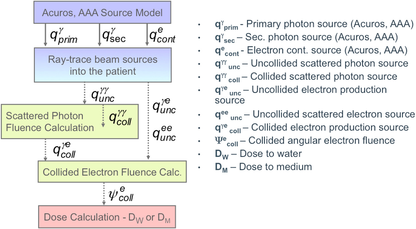
Acuros XB: Implementation and LBTE Discretisation
Acuros XB (External Beam), originally developed by Transpire Inc. and acquired by Varian for integration into Eclipse, solves the LBTE through a carefully ordered cascade of steps. The implementation decomposes the transport problem into components that are solved sequentially.
Step 1: Uncollided Photon Transport
The primary fluence — photons that have not undergone any interaction — is calculated by analytical ray-tracing from the accelerator source model. Each ray is attenuated exponentially as it traverses the patient voxels, using the macroscopic cross-sections of the material assigned to each voxel. The attenuation follows:
$$\psi_\gamma^{unc}(\vec{r}, E, \hat{\Omega}) = \psi_\gamma^{src}(E, \hat{\Omega}) \cdot \exp\left(-\int_0^s \sigma_{t,\gamma}(\vec{r}’, E)\, ds’\right)$$
Where $s$ is the distance travelled along direction $\hat{\Omega}$ from the source to point $\vec{r}$.
Step 2: Angular Discretisation — Discrete Ordinates ($S_N$)
The angular variable $\hat{\Omega}$ is discretised using the discrete ordinates ($S_N$) method. The unit sphere of directions is subdivided into a finite set of directions $\hat{\Omega}_n$ with quadrature weights $w_n$, so that integrals over solid angle are approximated by:
$$\int_{4\pi} f(\hat{\Omega})\, d\hat{\Omega} \approx \sum_{n=1}^{N_{dir}} w_n\, f(\hat{\Omega}_n)$$
Acuros XB typically uses quadrature sets with 80 to 128 discrete directions — sufficient to capture transport anisotropy in radiotherapy beams, including lateral scatter and backscatter.
Step 3: Energy Discretisation — Multigroup Method
The continuous energy spectrum is divided into discrete groups ($G$ groups typically). For each group $g$, cross-sections are pre-computed and tabulated as constants $\sigma_{t,g}$ and $\sigma_{s,g’ \to g}$. The transport equation for group $g$ in direction $\hat{\Omega}_n$ becomes:
$$\hat{\Omega}_n \cdot \nabla \psi_g^n(\vec{r}) + \sigma_{t,g}(\vec{r})\, \psi_g^n(\vec{r}) = \sum_{g’=1}^{G} \sum_{n’=1}^{N_{dir}} w_{n’}\, \sigma_{s,g’ \to g}(\vec{r}, \hat{\Omega}_{n’} \to \hat{\Omega}_n)\, \psi_{g’}^{n’}(\vec{r}) + q_{ext,g}^n(\vec{r})$$
The multigroup cross-section structure is derived from standard nuclear data libraries (similar to those used in nuclear reactor physics), adapted for energies of interest in radiotherapy (keV to MeV). Patient materials are assigned from CT densities using HU-to-material conversion tables with known chemical compositions.
Step 4: Spatial Discretisation — Finite Differences on the Patient Grid
The patient volume is discretised on the Eclipse calculation grid (typically 2.5 mm resolution, though fine resolution down to 1 mm is available). For each voxel, the multigroup discrete-ordinates equations are solved using finite-difference schemes that ensure particle conservation and fluence positivity.
The spatial sweep proceeds octant by octant: for each discrete direction $\hat{\Omega}_n$, voxels are swept in upstream-to-downstream order, so the incident fluence on each voxel has already been calculated from preceding voxels. This procedure is highly efficient and can be parallelised by octant.
Step 5: Scattered Photon Transport
The scattered photon source is computed from the uncollided photon fluence (Step 1). Compton, Rayleigh, and annihilation photons are transported iteratively: at each iteration, new scattered fluence contributes to a new scattering source, until convergence is reached.
Step 6: Electron Source and Electron Transport
Photoelectric, Compton, and pair production interactions generate secondary electrons. Acuros XB computes this electron source from the total photon fluence and then solves the LBTE for electrons, including continuous energy loss (CSDA) and bremsstrahlung production. The resulting electron fluence is integrated to produce the final dose distribution.
Source Model and Commissioning
Acuros XB uses the same multi-source virtual source model as AAA: primary source (target), extra-focal scatter source (flattening filter, collimators), and jaw/MLC transmission source. Parameters are fitted during commissioning from measured dosimetric data — PDDs, profiles, and output factors. This means clinics that have already commissioned AAA can migrate to Acuros XB without additional measurements.
Detailed Comparison: Monte Carlo vs. Acuros XB
The table below presents a direct comparison between Monte Carlo and Acuros XB across the aspects most relevant to clinical practice:
| Aspect | Monte Carlo | Acuros XB |
|---|---|---|
| Method | Stochastic — random sampling of particle histories | Deterministic — numerical LBTE solution on discrete grid |
| Statistical noise | Present; decreases as $1/\sqrt{N}$. Requires ~$10^9$ histories for uncertainty < 1% | Absent. Error is discretisation-based (voxel size, angular quadrature, energy groups) |
| Calculation time (typical IMRT) | 5–30 min (GPU-accelerated) to hours (CPU) | 1–5 min (standard multi-core CPU) |
| Homogeneous medium accuracy | Reference (gold standard) | Equivalent to MC (< 1% difference) |
| Lung accuracy | Reference | Within 1–2% of MC in most scenarios |
| Bone accuracy | Reference | Within 1–2% of MC |
| Air–tissue interfaces | Excellent (resolves CPE disequilibrium) | Excellent (solves LBTE explicitly) |
| Small fields (< 3×3 cm²) | Excellent | Excellent |
| $D_w$ / $D_m$ reporting | Both (native $D_m$) | Both (native $D_m$) |
| Metallic implants | Excellent (actual material composition) | Good (material assignment limited to library materials) |
| Magnetic field effects (MR-LINAC) | Excellent (EGSnrc, GEANT4 with magnetic extension) | Supported in Acuros XB v15.6+ for Unity (Elekta) |
| Very complex geometries | Superior (no angular discretisation approximations) | Good (finite angular resolution may smooth details) |
| Research and non-standard scenarios | Full flexibility (arbitrary geometries, custom scoring) | Limited to what the TPS offers |
| Commercial TPS | Monaco, iPlan, Oncentra, XiO, Pinnacle | Eclipse (Varian) — exclusive |
Advanced Clinical Applications of Acuros XB
Lung Stereotactic Body Radiotherapy (SBRT)
In lung SBRT, fields are small, heterogeneities are extreme (air to tumour to air), and charged particle equilibrium (CPE) does not exist at tumour boundaries. Studies such as Bush et al. (2011) and Fogliata et al. (2011) demonstrated that Acuros XB agrees with Monte Carlo within 1–2% under these conditions, while AAA can overestimate tumour coverage by up to 5–10% depending on lung density and field size. Acuros XB reporting dose-to-medium ($D_m$) correctly captures dose reduction at air–tumour interfaces.
MR-LINAC Treatment Planning
MR-LINAC systems such as Unity (Elekta) and ViewRay MRIdian generate a 0.35–1.5 T magnetic field that deflects secondary electron trajectories via the Lorentz force. This alters dose distributions, especially at air–tissue interfaces — the so-called electron return effect (ERE). Acuros XB version 15.6+ for Eclipse includes a magnetic field extension, solving the LBTE with additional deflection terms. The Lorentz force modifies the electron transport operator:
$$\hat{\Omega} \cdot \nabla \psi_e + \sigma_{t,e}\, \psi_e + \frac{e}{p}(\vec{v} \times \vec{B}) \cdot \nabla_{\hat{\Omega}} \psi_e = q_e$$
Where $\vec{B}$ is the magnetic field, $\vec{v}$ the electron velocity, $e$ the elementary charge, and $p$ the momentum. The additional $\nabla_{\hat{\Omega}}$ term represents rotation of the flight direction in angular space — essential for correctly capturing the ERE.
High-Density Metallic Implants
Hip prostheses (titanium, cobalt-chrome), dental implants, and fiducial markers introduce extreme heterogeneities (high effective $Z$, density 4–8 g/cm³). Acuros XB assigns material compositions from HU-to-material tables and computes material-specific cross-sections. For implants with very high density (above the typical CT range), assignment may be limited by the Acuros material library. In such cases, Monte Carlo with explicit implant geometry may be preferable.
Head and Neck: Bone–Air Interfaces
Tumours in nasal cavities, paranasal sinuses, and skull base involve frequent interfaces between bone, air, and soft tissue. Acuros XB captures backscatter effects and equilibrium loss at these interfaces with much greater accuracy than AAA — and with calculation times compatible with IMRT/VMAT inverse optimisation.
Why Acuros XB Is Replacing AAA in Eclipse
Since Eclipse version 13.6, Varian has positioned Acuros XB as the preferred photon algorithm. The reasons are clear:
- Accuracy: solves the LBTE explicitly, capturing heterogeneities with MC-level precision.
- Speed: 2–5x faster than MC for typical VMAT plans.
- No noise: deterministic result, free from sub-sampling artefacts.
- Dose-to-medium: reports $D_m$ natively, aligned with current recommendations.
- Simplified commissioning: uses the same source model as AAA.
In practice, departments migrating from AAA to Acuros XB often observe clinically relevant differences (2–5%) in lung plans, especially in SBRT with small fields. This difference can affect PTV coverage and OAR dose limits, justifying recalibration of institutional protocols.
Full Comparison: Monte Carlo vs Acuros vs Analytical Algorithms
| Feature | Monte Carlo | Acuros XB (LBTE) | AAA/CCC | Pencil Beam |
|---|---|---|---|---|
| Principle | Stochastic simulation | Deterministic LBTE solution | Convolution/Superposition | 1D convolution + corrections |
| Heterogeneity accuracy | Reference (gold standard) | Excellent (~1–2% of MC) | Good (CCC > AAA) | Limited |
| Small fields | Excellent | Excellent | Good (with limitations) | Poor |
| Computation time | Minutes–hours | Minutes | Seconds–minutes | Seconds |
| Statistical noise | Present (decreases with more histories) | Absent | Absent | Absent |
| $D_w$ vs $D_m$ | Both (native $D_m$) | Both | $D_w$ (native) | $D_w$ (native) |
| Available TPS | Monaco, iPlan, Oncentra, XiO | Eclipse (Varian) | Eclipse (AAA), Oncentra (CCC) | Various (legacy) |
Compiled from Handbook of Radiotherapy Physics: Theory and Practice, 2nd Ed. (CRC Press, 2020)
The Future of Dose Calculation
The convergence of ever-cheaper hardware — GPUs with thousands of cores, multithread processors, cloud computing — is making MC clinically viable for daily routine. The AAPM TG-157 report (2020) already considers MC the gold standard for electron beams and approaching full feasibility for photons.
In practice, two scenarios coexist. For clinics using Eclipse, Acuros XB offers the best accuracy–speed balance for photon dose calculation — especially in lung, head-and-neck, and stereotactic cases. For departments running Monaco or other XVMC/VMC++-based TPS platforms, Monte Carlo is already part of the routine with acceptable calculation times.
The AAPM TG-268 report (2018) established guidelines for reporting MC-based studies, standardising documentation of parameters such as energy cutoffs, VRTs used, and statistical uncertainties. This standardisation is essential for ensuring reproducibility and comparability between studies — and for reliably translating research findings into clinical practice.
The future points towards hybrid algorithms combining the deterministic robustness of Acuros with GPU acceleration and deep learning techniques for initial dose estimation, further reducing calculation time without compromising accuracy. GPU-accelerated Monte Carlo research projects (such as gDPM and ARCHER) have already demonstrated complete VMAT plan calculations in under 1 minute, bringing MC closer to real-time feasibility for adaptive radiotherapy.
To explore other aspects of Monte Carlo in radiotherapy, including applications in proton therapy, brachytherapy, and advanced QA, see our dedicated articles. For a comprehensive introduction to the Monte Carlo method in radiotherapy, see our complete Monte Carlo guide. And to understand how empirical dose calculation methods paved the way for these sophisticated techniques, read our algorithm evolution analysis.
This article is part of our series on photon dose calculation algorithms.