Empirical dose calculation methods — commonly known as broad-beam methods — formed the backbone of computerized radiotherapy treatment planning for decades. Before convolution algorithms and Monte Carlo became practical, medical physicists relied on tabulated beam data and semi-analytical corrections to estimate patient dose. This article covers each technique in depth: from the Bentley-Milan tabular representation to inhomogeneity corrections using Batho’s power-law, ETAR, and beam subtraction.
For a panoramic view of all photon dose calculation algorithms — from empirical to Monte Carlo — see our comprehensive guide on photon dose calculation algorithms.
Dose Components in Clinical Photon Beams
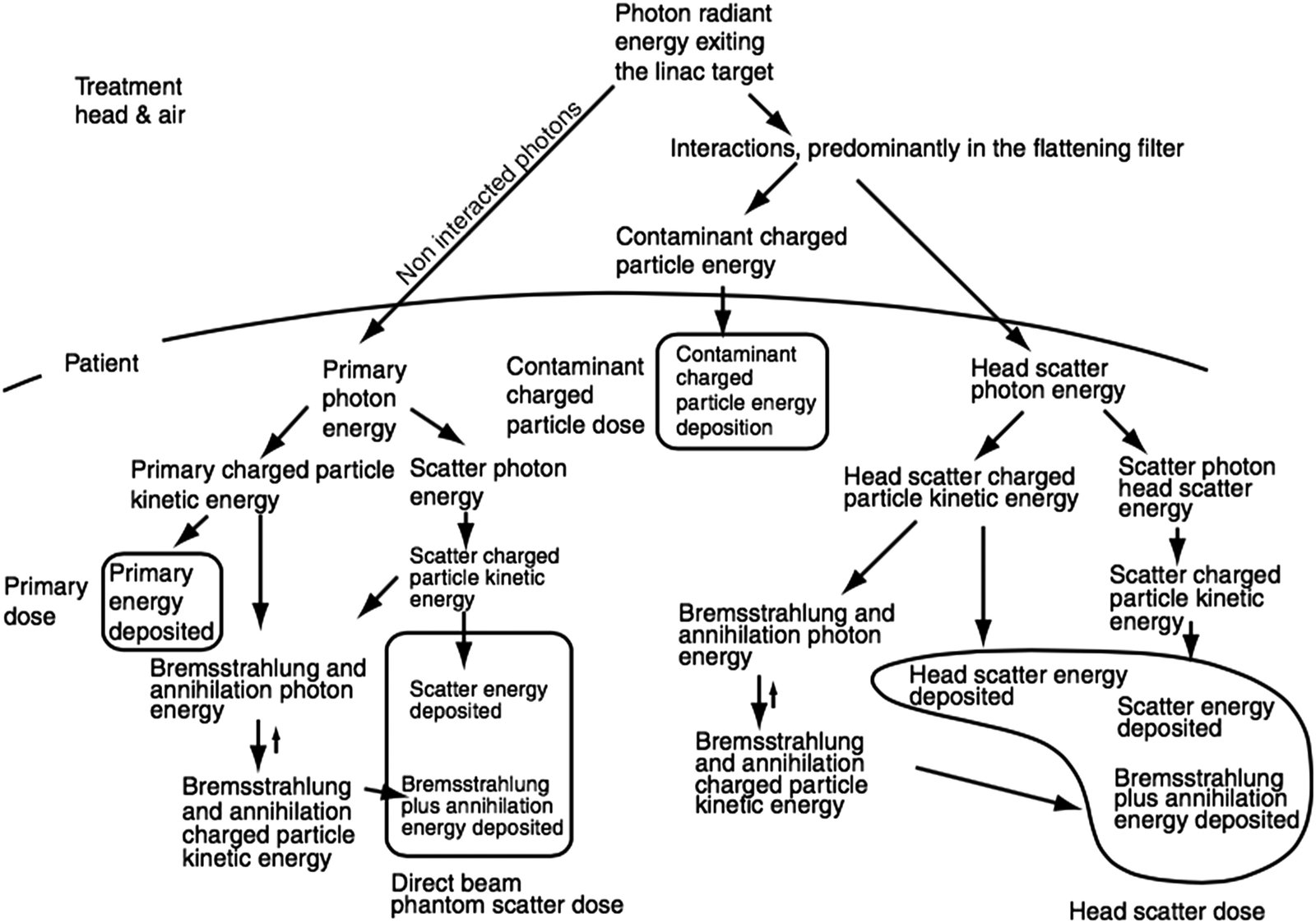
The total dose at any point in the patient arises from four distinct components. Primary dose, from photons emitted by the target without further interaction, typically accounts for over 70% of the total. Phantom scatter contributes up to 30%, depending on field size and depth.
Less obvious but clinically relevant, head scatter (the extrafocal contribution) — photons scattered in the flattening filter and collimator — can amount to 5–10% of total dose. Finally, contaminant charged particles, mostly electrons from photon interactions in head components and air, affect primarily the build-up region (typically the first 4 cm).
Broad-beam methods handle these components implicitly, without explicit separation. This simplification is both their strength — computational speed — and their fundamental weakness.
Tabulated Representations: The Bentley-Milan Model
In the 1970s, Bentley and Milan developed one of the first digital treatment planning systems. Their model stored beam data as central-axis depth-dose curves and off-axis ratios (OARs). To save memory — a critical constraint at the time — equivalent squares reduced arbitrary rectangular fields to square-field data.
Each square field had PDD curves stored at just 17 depths, equally spaced starting from $z_{max}$. The build-up region used a crude model: dose at depth $z < z_{max}$ was linearly interpolated between surface dose and maximum dose, using a modified depth $z_B$:
$$z_B = z_{max} – \frac{(z_{max} – z)^3}{z_{max}^2}$$
Off-axis ratios depended mainly on in-plane field width. Since their variation with depth was slow along divergent fan lines, only 5 storage depths sufficed. The original implementation fit the entire dataset into 255 items — exactly $2^8 – 1$.
Analytical Representations and Wedge Corrections
An alternative to tables was analytical fitting. Van de Geijn’s model (1965, 1970, 1972) split the beam representation into central-axis depth-dose and off-axis ratios, each modeled by a mathematical function. Only seven measurements were needed to characterize PDD curves for a given energy — a huge saving in commissioning time.
For wedge filters, two approaches coexisted. The first included wedged dose distributions directly in the experimental dataset. The second derived a transmission profile from measurements with and without wedge in a large field, tabulating it as a correction factor. In practice, this profile could also be calculated from filter dimensions and composition, provided the attenuation coefficient was experimentally verified. The wedge transmission concept is not limited to the broad-beam approach and has been adopted by more modern algorithms.
Patient Shape Correction: Effective SSD and TPR Methods
The human body is not a flat water block. Correcting dose for real surface curvature requires dedicated methods.
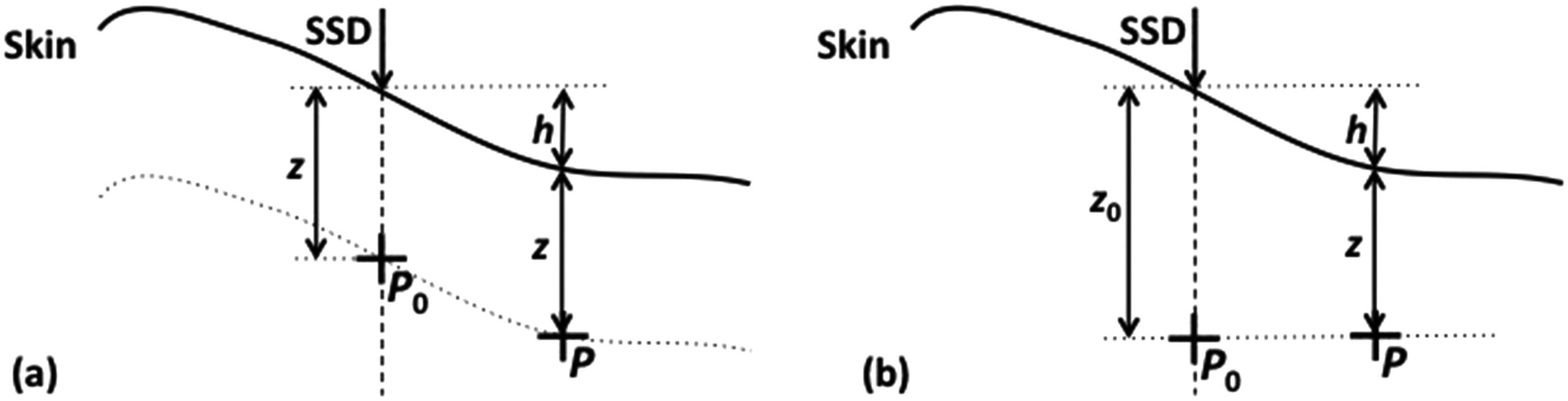
Effective SSD Method
The effective SSD method applies an inverse square law correction. If the central-axis SSD is $SSD$ and the increase in distance for an off-axis point is $h$, the correction factor is:
$$C_{SSD} = \left(\frac{SSD + z}{SSD + h + z}\right)^2$$
In the Bentley-Milan approach, measured data were first converted to “infinite SSD” (removing inverse-square variation), then the geometric correction was applied for the actual treatment SSD.
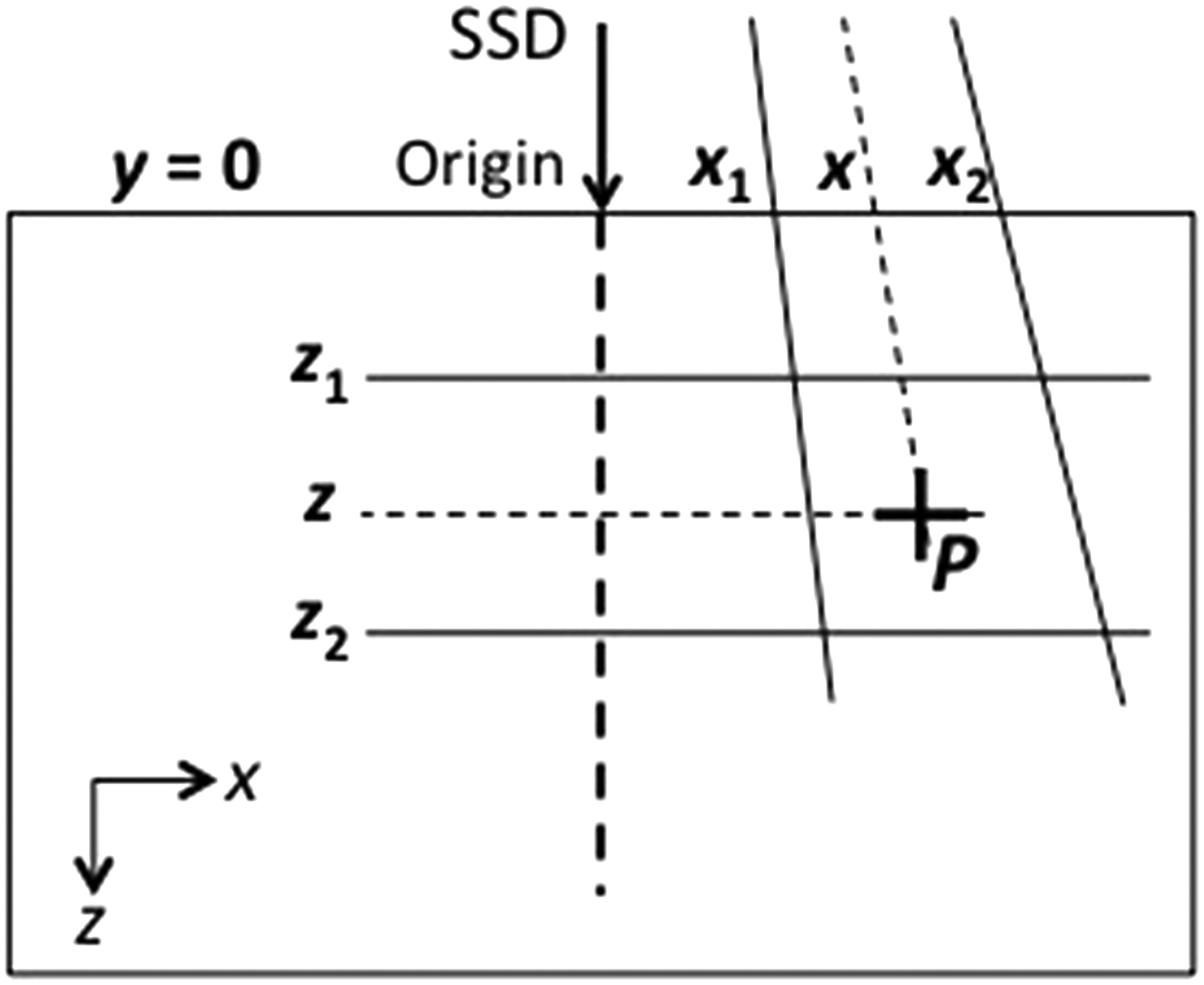
TPR Ratio Method
An alternative is the TPR ratio method. The correction factor is the ratio of two tissue phantom ratios, which are independent of SSD:
$$C_{TPR} = \frac{TPR(z, ESQ_{z_0})}{TPR(z + h, ESQ_{z_0})}$$
In both cases, an additional off-axis correction accounts for the flattening filter and wedge.
Inhomogeneity Corrections: From Effective Depth to Batho
The presence of lung, bone, and air in the beam path changes both attenuation and scatter. Broad-beam methods developed progressively more sophisticated corrections.
Effective Depth (TAR)
The simplest method replaces real depth with an effective depth $z_{eff}$, the water-equivalent thickness along the fan line:
$$z_{eff} = \sum_{i=1}^{n} t_i \, \rho_i$$
The correction factor uses TAR (or TPR) ratios:
$$C_{het}^{TPR} = \frac{TPR(z_{eff}, ESQ_z)}{TPR(z, ESQ_z)}$$
This is a one-dimensional correction that ignores lateral scatter changes — acceptable far from the inhomogeneity, but insufficient at interfaces.
Batho Power-Law Correction
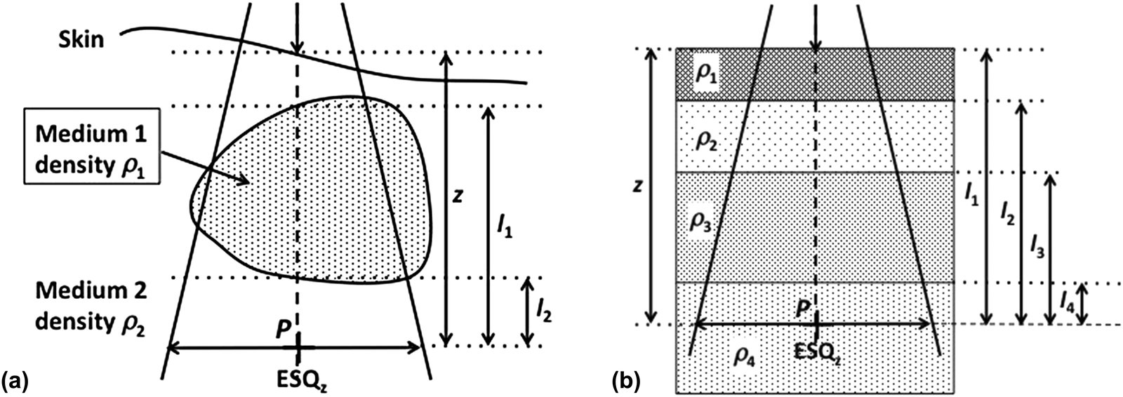
The power-law method, proposed by Batho (1964) and generalized by Sontag and Cunningham (1977), raises the TAR to the power of the medium’s relative density. For a point $P$ in medium of density $\rho_2$ below an inhomogeneity of density $\rho_1$:
$$C_{het}^{Batho} = TAR(l_2, ESQ_z)^{(\rho_2 – \rho_1)} \cdot TAR(l_1, ESQ_z)^{(1 – \rho_1)}$$
For multiple superimposed layers, Webb and Fox’s (1980) generalization is:
$$C_{het}^{Batho} = \prod_{i=1}^{n} TAR(l_i, ESQ_z)^{(\rho_i – \rho_{i-1})}$$
where $l_i$ is the distance from point $P$ to the distal boundary of the $i$-th inhomogeneity and $\rho_0 = 1$.
Experimental Comparison of Methods
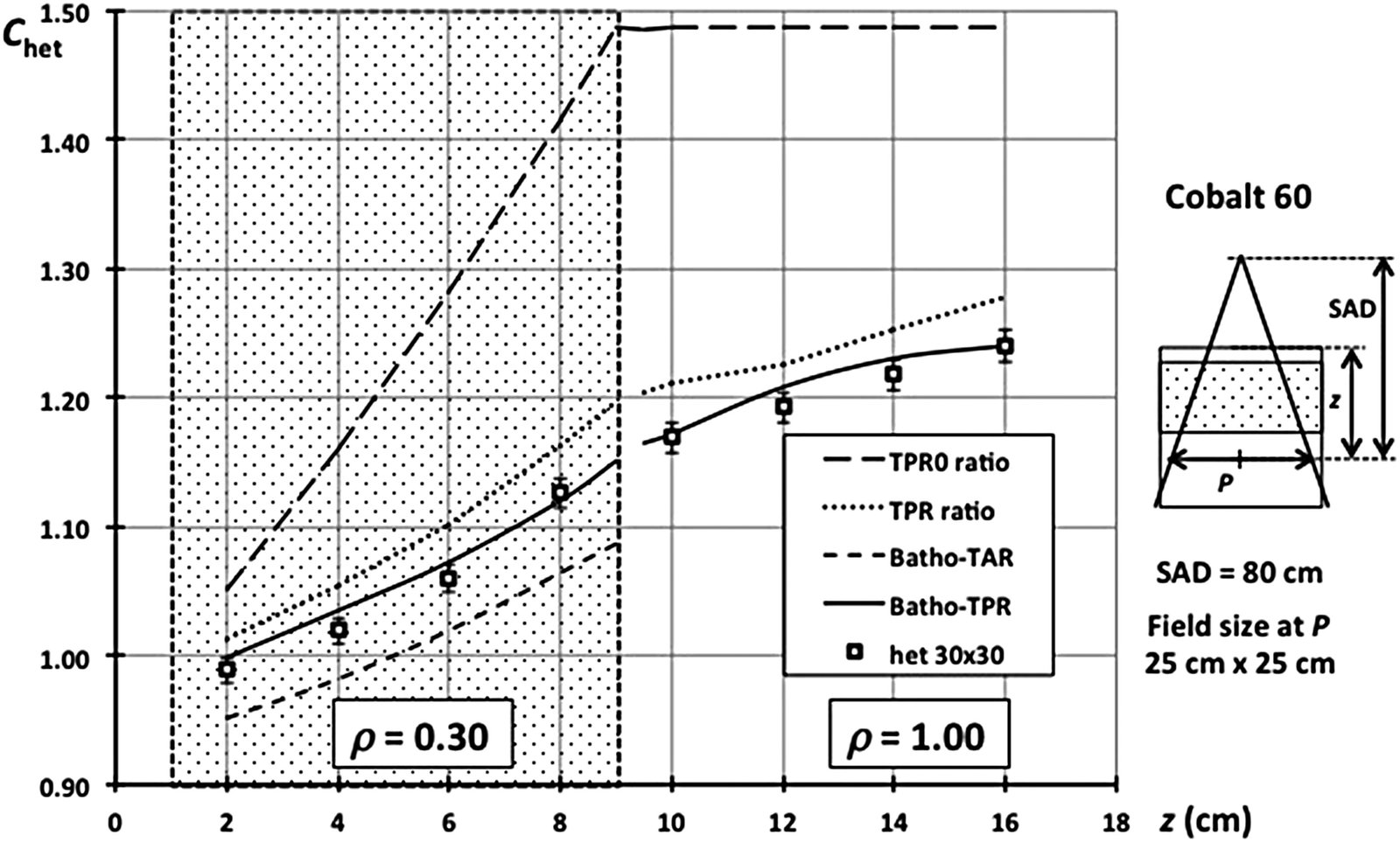
Figure 28.5 shows results for an 8 cm thick inhomogeneity ($\rho = 0.3$) at 1 cm depth in a cobalt-60 beam. The TPR0 (primary-only) method grossly overestimates the correction. The full TPR ratio improves but still overestimates within the inhomogeneity. The original Batho correction (TAR-based) works well below the inhomogeneity but underestimates within it. The Batho-TPR formulation, using TPR ratios, provides the best compromise across all regions — with errors typically under 2% in water below low-density layers.
| Method | Within inhomogeneity | Below inhomogeneity | Main limitation |
|---|---|---|---|
| Effective depth (TAR/TPR ratio) | Overestimates correction | Overestimates correction | Ignores scatter modification |
| Original Batho (TAR) | Underestimates dose | Good accuracy (~2%) | No backscatter accounting |
| Modified Batho-TPR | Best result | Good accuracy (~2%) | Assumes slab geometry |
| Batho-TPR (zero field) | Equivalent to TAR ratio | Equivalent to TAR ratio | Only valid for small fields |
Source: Handbook of Radiotherapy Physics, 2nd Ed., Chapter 28
Critical points Batho cannot resolve: for high-density inhomogeneities ($\rho > 1$), accuracy drops. At high energies, electronic equilibrium may fail — invalidating the local energy deposition assumption. And the multiplicative layer-by-layer application is often too crude.
Beam Subtraction and ETAR: 3D Refinements
Beam Subtraction Method
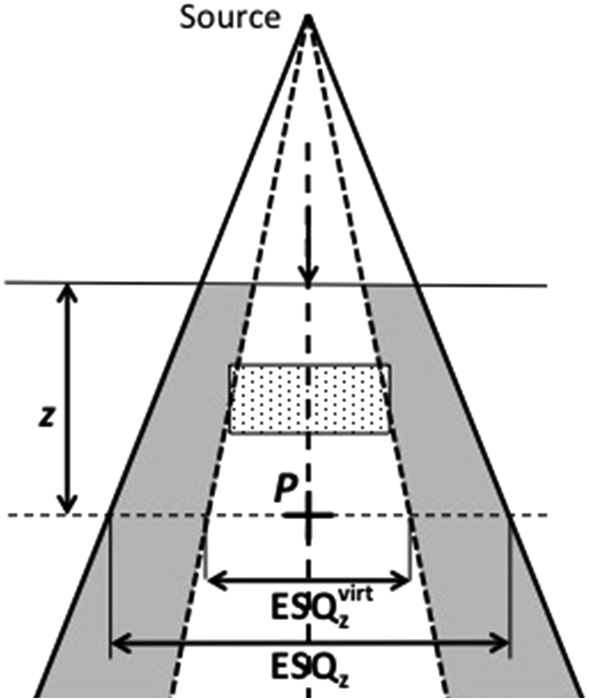
When the inhomogeneity is smaller than the field, Batho’s method fails because it assumes infinite slab geometry. Beam subtraction (Lulu and Bjärngard, 1982; Kappas and Rosenwald, 1982) addresses this by using a virtual beam ($ESQ_z^{virt}$) that exactly covers the inhomogeneity:
$$C_{het}^{Batho-subt} = 1 + \frac{TPR(z, ESQ_z^{virt})}{TPR(z, ESQ_z)} \times (C_{het}^{Batho} – 1)$$
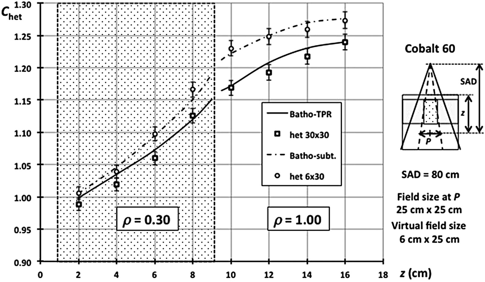
Figure 28.7 confirms the effectiveness: for a 6 cm wide inhomogeneity ($\rho = 0.3$) in a 25×25 cm² field, the beam subtraction curve matches the experimental data points. The scatter deficit within and below the inhomogeneity is naturally smaller for 6 cm width compared to 30 cm.
ETAR Method (Equivalent Tissue-Air Ratio)
The ETAR method (Sontag and Cunningham, 1978) goes further by scaling not only depth but also field size. The correction factor becomes:
$$C_{het}^{ETAR} = \frac{TPR(z_{eff}, ESQ_z^{eff})}{TPR(z, ESQ_z)}$$
where $ESQ_z^{eff}$ results from scaling the equivalent circular field radius by the effective density $\bar{\rho}$, computed as a weighted average of voxel-by-voxel densities from CT:
$$\bar{\rho} = \frac{\sum_{i,j,k} \rho_{ijk} W_{ijk}}{\sum_{i,j,k} W_{ijk}}$$
The weights $W_{ijk}$ represent each voxel’s scatter contribution at the calculation point. At the time, full 3D computation was prohibitive, so Sontag and Cunningham reduced the density array to 2D by collapsing pixels with the same X,Z coordinates. This simplification introduced inconsistencies documented by Wong and Henkelman (1983).
Limitations of Broad-Beam Methods
After traversing the entire correction chain — shape, inhomogeneity, field size — it becomes clear why broad-beam methods were progressively replaced. Each correction adds approximations on top of approximations. They worked reasonably for rectangular fields and served as the clinical standard for decades, but are inadequate for modern scenarios: non-rectangular fields, IMRT, VMAT, and stereotactic treatments.
The fundamental limitation is treating scatter globally, without explicit ray-tracing of the scatter component. Applying corrections designed for large slabs to voxel-sized inhomogeneities (such as bone-soft tissue interfaces in vertebrae) produces clinically relevant errors.
Computer speed removed the original motivation: resource economy. Monte Carlo and convolution/superposition algorithms now offer fundamentally superior accuracy with acceptable clinical calculation times. For a complete overview of this evolution, see our guide on photon dose calculation algorithms.