Energy Deposition Kernels and Collapsed Cone Convolution: Complete Theory and Clinical Implementation

Collapsed Cone Convolution: the physics behind modern dose calculation

The Collapsed Cone Convolution (CCC) algorithm stands as one of the most important advances in photon dose calculation for radiation therapy. Proposed by Ahnesjö in 1989, CCC addresses a practical problem that challenged medical physicists for years: how to accurately compute dose in heterogeneous media without the prohibitive computational cost of full point-by-point superposition? The answer lies in a clever combination of energy deposition kernels with a geometric approximation that collapses transported energy onto discrete cones. For a comprehensive overview of dose calculation algorithms, from empirical methods to Monte Carlo, see our complete guide on photon dose calculation algorithms.

This article presents an exhaustive analysis of the three landmark papers that defined CCC: the Monte Carlo energy deposition kernels (Mackie et al., 1988), the collapsed cone convolution method (Ahnesjö, 1989), and the practical treatment planning system implementation (Cho et al., 2012). We also discuss commercial implementations in systems such as Pinnacle (Philips), Oncentra (Elekta), and RayStation (RaySearch), and compare CCC against other dose calculation algorithms.

Historical Context: Why CCC Was Needed

In the 1980s, radiation therapy dose calculation relied on empirical methods based on measured percentage depth dose (PDD) tables and lateral profiles in water. These methods — such as Clarkson’s integration algorithm for irregular fields — worked reasonably for simple geometries in homogeneous media, but could not handle the anatomical reality of patients. Lung tissue, air cavities, cortical bone, and metallic implants profoundly alter radiation transport, and empirical methods applied only crude tissue-air ratio (TAR) or tissue-phantom ratio (TPR) corrections.

The fundamental issue was conceptual. In a homogeneous water medium, the dose at any point can be calculated by convolution: the primary photon fluence is convolved with a kernel describing how energy redistributes after each interaction. Mackie et al. (1985) formalized this mathematically. However, in heterogeneous media, the kernel changes from point to point — depending on the density and composition of tissue between the interaction and deposition sites. Simple convolution becomes superposition, and computational cost rises from $n^3$ to $n^6$ operations, where $n$ is the number of voxels per dimension.

Full Monte Carlo simulation solved the problem accurately, but in 1989 a typical treatment plan would take hours or days on available hardware. Clinicians needed something in between: an algorithm that captured the physics of energy transport in heterogeneous media yet ran in minutes. Ahnesjö’s CCC filled that gap with an elegant solution — reducing complexity to $n^4 \times m$ operations through the collapsed cone approximation, without significantly sacrificing dosimetric accuracy.

Mackie 1988: EGS Monte Carlo Kernel Generation

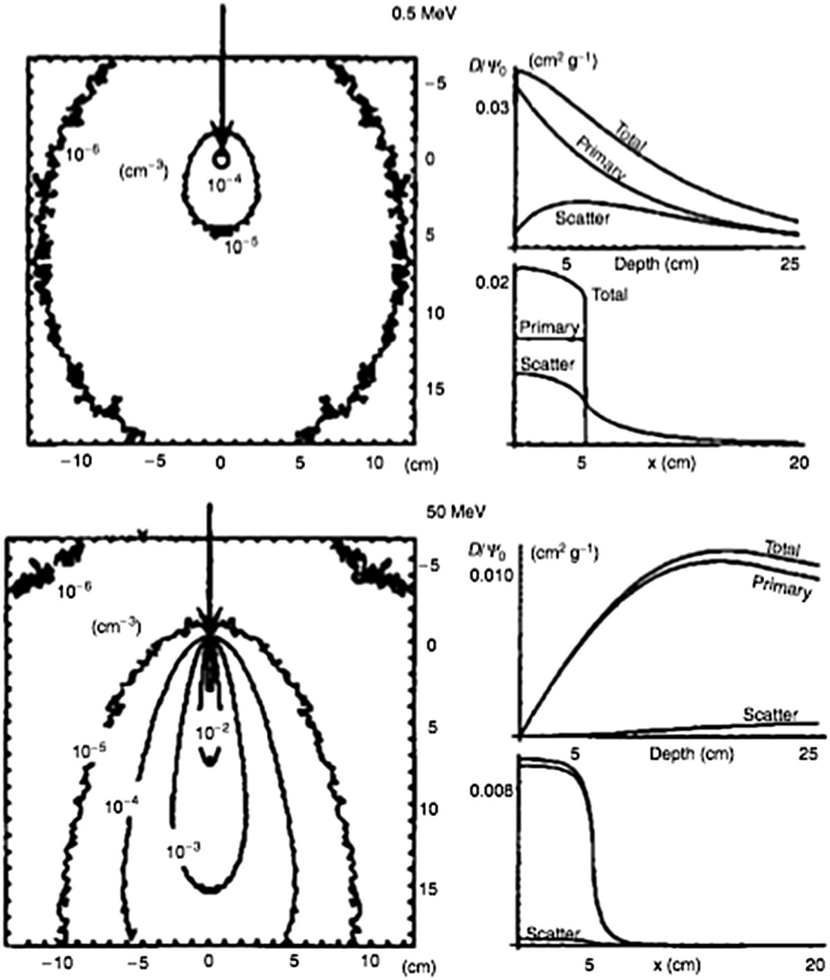
Energy deposition point kernels — also called dose spread arrays — are the central building block of any convolution/superposition algorithm. They describe how energy spreads through space around a primary photon interaction site. The landmark work by T.R. Mackie, J.W. Scrimger, J.J. Battista (1988) established the standard method for generating these kernels using Monte Carlo simulation.

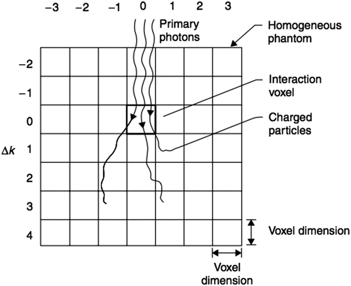
Simulation geometry

Mackie and colleagues used the EGS (Electron Gamma Shower) Monte Carlo code with a user code called SCASPH to simulate particle transport in a homogeneous spherical water phantom. The geometry was divided into:

• Angular cones of 3.75° aperture (48 cones covering 180°)
• 24 radial shells with increasing spacing
• Forced interaction at the exact center of the sphere

Monoenergetic photons were forced to interact at the sphere center. From this primary interaction, all secondary particles — Compton electrons, electron-positron pairs, photoelectrons, annihilation electrons, and bremsstrahlung photons — were tracked until losing all kinetic energy or escaping the phantom. The energy deposited in each voxel (defined by the cone-shell intersection) was recorded and accumulated over thousands of histories.

Kernels for different scattering orders

A key contribution of Mackie’s work was the decomposition of kernels by scattering order:

• Primary kernel ($K_p$): energy deposited by charged particles from the primary interaction (Compton, photoelectric, pair production)
• First-scatter kernel ($K_{s1}$): energy deposited after a single scattering interaction of the secondary photon
• Second-scatter kernel ($K_{s2}$): after two scattering interactions
• Multiple-scatter kernel ($K_{sm}$): all higher orders
• Bremsstrahlung and annihilation kernel ($K_{ba}$): photons generated by these processes

Kernels were calculated for monoenergetic photons from 0.1 to 50 MeV. Beyond deposition kernels, the work also characterized primary particle transport through parameters such as effective voxel center, penetration depth, effective radius, and effective lateral distance. These data served as the foundational database for all subsequent convolution/superposition algorithms, including CCC.

Normalization integrals

The total kernel decomposes into primary and scatter components. The normalization integrals satisfy:

$$\iiint K_p(\mathbf{r})\,dV = \frac{\mu_{en}}{\mu}$$

$$\iiint K_s(\mathbf{r})\,dV = \frac{\mu – \mu_{en}}{\mu}$$

Where $\mu$ is the total linear attenuation coefficient and $\mu_{en}$ is the linear energy-absorption coefficient. These relations are fundamental for verifying generated kernels and applying beam-quality corrections in clinical implementations.

Energy dependence

The figure illustrates kernels for 0.5 MeV and 50 MeV. The difference is dramatic. At low energies (below 1 MeV), scattered photon contributions dominate and the kernel is relatively isotropic — energy distributes almost uniformly in all directions. At high energies (above 10 MeV), electron transport becomes dominant and highly directional: energy deposits preferentially in the forward direction (same direction as the incident photon), with significant lateral electron ranges.

This energy-dependent behavior has profound practical consequences. For 6 MV beams, where the mean spectrum energy is around 2 MeV, kernels are moderately anisotropic and heterogeneity corrections have intermediate importance. For 15–18 MV beams, kernels are strongly anisotropic and failures of simple algorithms in lung and air cavities become clinically relevant. CCC, by transporting energy along discrete directions with density scaling, captures this anisotropy significantly better than pencil beam algorithms.

Analytical Representation and Polyenergetic Kernels

Working directly with tabulated kernels for each energy at each angle is computationally expensive and hinders recursive calculation. Ahnesjö and Mackie (1987) proposed an analytical fit that made CCC feasible:

$$K(r, \theta) = \frac{A_\theta\, e^{-a_\theta r} + B_\theta\, e^{-b_\theta r}}{r^2}$$

Where:

• $r = |\mathbf{r} – \mathbf{r}’|$ is the distance between interaction point $\mathbf{r}’$ and deposition point $\mathbf{r}$
• $\theta$ is the angle relative to the incident photon direction
• $A_\theta, a_\theta, B_\theta, b_\theta$ are fitting parameters depending on $\theta$ and the energy spectrum
• The $1/r^2$ factor compensates for geometric dispersion from a point source
• The first exponential primarily describes primary deposition (short range); the second describes the scatter component (long range)

The elegance of this formulation lies in enabling recursive calculation. If we know the accumulated dose up to position $r_i$ along a line, the contribution to $r_{i+1} = r_i + \Delta r$ can be obtained by multiplying by the corresponding exponential — without recalculating the entire integral. This property is what makes CCC computationally feasible.

Polyenergetic kernels for clinical beams

Clinical beams are not monoenergetic. A 6 MV beam contains photons from 0 to 6 MeV with a mean energy around 2 MeV. Furthermore, the spectrum changes with depth (beam hardening) and lateral position (off-axis softening). Two main approaches exist:

• Spectrum-weighted summation: polyenergetic kernels are generated by weighted summation of Mackie’s monoenergetic kernels using the incident fluence spectrum weights. This is the most straightforward method.
• Depth-based interpolation: Liu et al. (1997) proposed pre-calculating polyenergetic kernels at three distinct depths (shallow, intermediate, deep) and interpolating during calculation. This automatically compensates for beam hardening without recalculating the spectrum at each point.

A refined alternative convolves primary and scatter kernels separately with their respective TERMA fractions: $\mu_{en}/\mu$ for primary and $(\mu – \mu_{en})/\mu$ for scatter. Since each component responds differently to spectral changes, this separation improves accuracy without significant computational overhead.

Ahnesjö 1989: The Collapsed Cone Convolution Method

Anders Ahnesjö‘s 1989 paper in Medical Physics is the founding work of CCC. Ahnesjö proposed an elegant solution to the superposition problem in heterogeneous media, combining three innovations: ray-tracing for TERMA, analytical polyenergetic kernels, and the collapsed cone approximation.

TERMA calculation by ray-tracing

TERMA (Total Energy Released per unit MAss) describes the total energy released by photons at each volume point. Ahnesjö calculated TERMA by tracing rays from the photon source through the patient volume:

$$T(\mathbf{r}’) = \Psi(\mathbf{r}’) \cdot \frac{\mu(\mathbf{r}’)}{\rho(\mathbf{r}’)}$$

Where $\Psi(\mathbf{r}’)$ is the energy fluence at point $\mathbf{r}’$ (calculated by ray-tracing with exponential attenuation) and $\mu/\rho$ is the tissue mass attenuation coefficient at that point. Fluence is attenuated along the path considering tissue composition and density — inhomogeneities such as lung, bone, and air alter both attenuation and the resulting TERMA.

The collapsed cone approximation

Direct superposition requires integrating the contribution from all $n^3$ interaction voxels for each of the $n^3$ deposition voxels — $n^6$ operations total, rising to $n^7$ with variable scaling. CCC solves this by discretizing the angular space into $m$ fixed directions (typically 13 axes generating 26 senses, or more refined versions with 48 or more directions).

For each of these $m$ directions, all energy within a solid cone of solid angle $\Omega$ is collapsed (projected) onto the cone’s central axis. Energy is then transported and deposited step by step along this line, using the analytical kernel formulation. At each step, the calculation considers the local radiological density for kernel scaling.

The deposition equation along a cone direction $\hat{\Omega}_j$ can be written as:

$$D_j(\mathbf{r}) = \sum_{i} T(\mathbf{r}_i’) \cdot \Delta V_i \cdot \frac{\Omega_j}{4\pi} \cdot \frac{A_\theta e^{-a_\theta d_{\rho}} + B_\theta e^{-b_\theta d_{\rho}}}{d_{\rho}^2}$$

Where $d_{\rho}$ is the radiological distance (density-scaled) between $\mathbf{r}_i’$ and $\mathbf{r}$, and $\Omega_j/4\pi$ is the solid angle fraction covered by cone $j$. Total dose is the sum over all directions:

$$D(\mathbf{r}) = \sum_{j=1}^{m} D_j(\mathbf{r})$$

Thanks to the exponential kernel form, transport along each line can be calculated recursively. Denoting $E_j(\mathbf{r}_k)$ as the accumulated energy arriving at voxel $k$ along direction $j$, the next voxel’s contribution is:

$$E_j(\mathbf{r}_{k+1}) = E_j(\mathbf{r}_k) \cdot e^{-a_\theta \Delta d_{\rho}} + T(\mathbf{r}_k) \cdot \Delta V_k \cdot \frac{\Omega_j}{4\pi}$$

This recursion reduces total operations to $n^4 \times m$, where $n^3$ are the voxels and $n$ is the typical transport line length. In practice, with $m \sim 26$ to $48$ directions and grids of $128^3$ to $256^3$ voxels, complete calculation takes seconds to a few minutes on modern hardware.

Energy conservation in CCC

The collapsed cone approximation preserves energy conservation by construction. All energy emitted into each solid angle is assigned to the corresponding cone’s central axis. There is no net loss or gain — total deposited energy equals total released energy (integrated TERMA), respecting escape fractions when energy exits the patient volume.

Original validation

Ahnesjö validated CCC for accelerating potentials of 4, 6, 10, 15, and 24 MeV in two geometries:

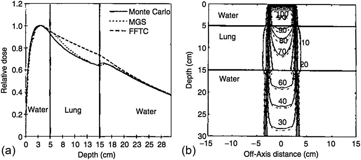
1. Layered tissue stack: water + lung + water, testing CCC’s ability to handle density interfaces
2. Mediastinal phantom: cork (simulating lung) and water, reproducing a clinically relevant geometry

Calculated dose distributions were compared against reference EGS4 Monte Carlo simulations. Agreement was excellent in both geometries and across the entire energy range tested. Ahnesjö demonstrated that the number of operations scales proportionally with calculation points — establishing clinical feasibility. The original paper notes that CCC can model both lateral electron transport at interfaces and differential attenuation in media of different densities, surpassing the primary-scatter correction algorithms available at the time.

Beam Divergence and Kernel Tilting

A real clinical beam diverges from the source. This divergence modifies not only fluence (inverse-square law) but also kernel directions: strictly, off-axis kernels should be tilted to follow divergence. In practice, Sharpe and Battista (1993) showed that keeping all kernels parallel to the central axis is acceptable for most clinical situations.

When does this break down? At short source-surface distances, large field sizes, and high energies. Replacing a tilted off-axis kernel with a parallel one increases its contribution to the beam axis, overestimating on-axis PDD. Papanikolaou et al. (1993) and Liu et al. (1997) proposed applying inverse-square correction at deposition points instead of interaction points as compensation. Ahnesjö et al. (2005) took a more explicit approach: using the analytical kernel form with fitting parameters dependent on the tilt angle.

Density Scaling and Tissue Inhomogeneities

Inhomogeneity handling is where CCC fundamentally distinguishes itself from simpler algorithms. If the medium density differs from water, O’Connor’s theorem states that the same dose distribution can be obtained by scaling all phantom dimensions proportionally. In practice, this is equivalent to replacing all distances in the convolution equation with radiological equivalent distances.

The general convolution equation in homogeneous medium reads:

$$D(\mathbf{r}) = \iiint T(\mathbf{r}’) \cdot K(\mathbf{r} – \mathbf{r}’)\,d^3\mathbf{r}’$$

In heterogeneous media, distances are scaled according to local density. Three regions must be considered separately:

• Density $\rho_1$ between the surface and $\mathbf{r}’$ — modifying fluence $\Psi(\mathbf{r}’)$ and therefore TERMA
• Density at $\mathbf{r}’$ — modifying TERMA via $\mu/\rho$
• Density $\rho_2$ between $\mathbf{r}’$ and $\mathbf{r}$ — modifying the kernel to $K(\rho_2 \cdot |\mathbf{r} – \mathbf{r}’|)$

In CCC, this scaling is naturally applied along each transport line. The radiological distance $d_\rho$ accumulates relative density voxel by voxel: $d_\rho = \sum_i \rho_i \cdot \Delta s_i$, where $\Delta s_i$ is the geometric length in voxel $i$ and $\rho_i$ is its density relative to water. This accumulation allows the exponential kernel to adjust automatically: in lung ($\rho \approx 0.3$), radiological distance grows more slowly than geometric distance, making the kernel decay more slowly and energy penetrate deeper — exactly what happens physically.

Even with full scaling, the convolution equation in heterogeneous media remains approximate. For the primary kernel, rectilinear scaling is not exact regarding multiple scattering of secondary electrons. For the scatter kernel, rectilinear scaling is rigorous only for the first-scatter component. Mackie et al. (1985) suggested separating first-scatter from multiple-scatter kernels, scaling the latter based on an average density value. Since the multiple-scatter component is a small dose fraction — especially at high energy — using the same density value for all scatter is also acceptable in clinical practice.

Cho 2012: Practical Implementation with Three-Source Model

The paper by Woong Cho, Kwangzoo Chung and colleagues (2012), published in the Journal of the Korean Physical Society, details how to transform CCC theory into a functional treatment planning system. While Ahnesjö defined the mathematical framework, Cho demonstrated the practical implementation details.

Three-source fluence model

The first practical challenge is determining the photon fluence entering the patient. Cho used a three-source model:

1. Primary source (target): bremsstrahlung photons from the linear accelerator target. Angular and energy distributions are characterized by parameters fitted from water PDD and profile measurements.
2. Primary collimator scatter: photons interacting with jaws and primary collimator before reaching the patient. These contribute to fluence broadening beyond the defined field edge.
3. Additional gantry head scatter: photons scattered by the flattening filter, accessory tray, and other head structures. These contribute to out-of-field dose and lateral profile shape.

This multi-source model is more accurate than a simple point-source model, especially for large fields and for reproducing the horn effect (fluence increase at field edges caused by the conical flattening filter). Model parameters are fitted during accelerator commissioning using PDD, lateral profile, and output factor measurements across different field sizes.

TERMA calculation with physical effects

TERMA in Cho’s work incorporates several physical effects neglected in simplified implementations:

• Polyenergetic spectrum: attenuation calculated using energy-dependent coefficients weighted by the local spectrum
• Horn effect: radial fluence variation caused by the conical flattening filter
• Beam softening: mean spectrum energy decreases off-axis and increases with depth
• MLC transmission: attenuation through multileaf collimator leaves, including interleaf leakage and tongue-and-groove effects
• Medium attenuation: exponential fluence reduction through the patient, calculated by voxel-by-voxel ray-tracing

Collapsed cone line convolution

Dose was calculated by convolving TERMA with a polyenergetic kernel approximated by dozens of collapsed cone lines. Cho typically implemented 26 to 48 discrete directions. In each direction, energy deposition follows the recursive formulation described in the Ahnesjö section, with voxel-by-voxel density scaling.

Validation against film dosimetry

Cho’s experimental validation is particularly relevant because it uses film dosimetry under realistic conditions:

• PDDs (Percentage Depth Dose): calculated and measured for 5×5 to 20×20 cm² fields at 6 and 15 MV
• Lateral profiles: at multiple depths, verifying penumbra, flatness, and out-of-field dose
• Pencil beam comparison: CCC was also compared with a pencil beam algorithm implemented in the same system

Results showed agreement within 2% between CCC and film measurements for the vast majority of points, except in the build-up region. In this region (first few millimeters), empirical electron contamination modeling and the transition to electronic equilibrium are analytically difficult to capture, resulting in larger discrepancies. Cho noted that CCC significantly outperformed pencil beam in heterogeneous situations, confirming the theoretical advantage predicted by Ahnesjö.

Commercial TPS Implementations

CCC has been adopted by multiple treatment planning system manufacturers. Each implementation has particularities, but all follow the framework established by Mackie, Ahnesjö, and validated by Cho:

Philips Pinnacle³

Pinnacle was the first commercial TPS to implement CCC as its primary dose calculation algorithm. Developed from Mackie et al.’s original work at the University of Wisconsin, Pinnacle uses Mackie’s kernels with Ahnesjö’s collapsed cone formulation. Historically considered the “gold standard” among convolution/superposition algorithms, Pinnacle typically uses 26 to 80 cone directions, with options to increase for complex geometries.

Elekta Oncentra (formerly Helax-TMS)

Oncentra Masterplan has a direct connection to Ahnesjö, who participated in developing Helax-TMS in Sweden. The implementation closely follows the original 1989 paper. When Elekta acquired Nucletron and later integrated Helax, Oncentra’s CCC was maintained as a reference algorithm.

RayStation (RaySearch Laboratories)

RayStation offers both CCC and Monte Carlo. RayStation’s CCC is a modern implementation leveraging multi-core parallelization and algorithmic optimizations to achieve calculation times of seconds on typical grids. It is frequently used as the fast calculation algorithm during inverse IMRT/VMAT optimization, with final verification by Monte Carlo.

XiO and Monaco (Elekta)

XiO (originally CMS Focus) used CCC as its primary algorithm for many years. Monaco, XiO’s successor, migrated to GPU-based Monte Carlo as its primary algorithm but still uses convolution/superposition principles in specific modules.

ISOgray (DOSIsoft)

ISOgray implements CCC with a formulation close to Ahnesjö’s original, being widely used in Europe, particularly in France and French-speaking countries.

Electron contamination and exit dose

Point-kernel convolution covers all voxels in the patient volume, allowing surface obliquity effects to be modeled. However, electron contamination from the treatment head and air is not captured by the kernels. This is handled through an additional empirical dose component dependent on SSD, field size, and off-axis distance, decreasing exponentially from the surface to the maximum contaminant electron range. On the patient exit side, since there is no kernel contribution from air, a slight dose overestimation occurs — a minor effect in most clinical cases.

Comparison Table: CCC vs Pencil Beam vs AAA vs Monte Carlo

The table below compares the main photon dose calculation algorithms available in commercial treatment planning systems. The inclusion of Varian’s AAA (Analytical Anisotropic Algorithm) and Acuros XB complements the comparison with widely used clinical algorithms.

Feature	Pencil Beam	CCC / Superposition	AAA (Varian)	Acuros XB	Monte Carlo
Theoretical basis	2D convolution with invariant kernels	3D superposition with collapsed cones	Superposition with separate anisotropic kernels	Boltzmann transport equation (LBTE)	Stochastic particle-by-particle simulation
Calculation order	$n^3$ (2D conv.)	$n^4 \times m$	$n^4 \times m’$	Deterministic, proportional to $n^3$	Stochastic ($N_{hist}$ particles)
Inhomogeneities	Type-a correction (depth scaling)	3D density scaling	Density scaling with separate kernels	Explicit multi-material transport	Explicit transport, exact
Lateral electron transport	Not modeled	Approximate (rectilinear scaling)	Approximate (better than PB)	Yes (deterministic resolution)	Yes (complete)
Lung penumbra	Underestimates broadening	Reasonable (±3–5%)	Reasonable (±2–4%)	Accurate (±1–2%)	Exact (reference)
Air-tissue interface dose	Inaccurate	Good for most cases	Good for most cases	Accurate	Exact
Build-up	Empirical	Empirical (±2–5%)	Empirical (±2–5%)	Better (±1–3%)	Exact
Typical speed	Seconds	Seconds to minutes	Seconds to minutes	Minutes	Minutes to hours
GPU / parallelization	Not needed	Supported (RayStation, Monaco)	Supported (Eclipse)	Yes (Eclipse)	Essential (Monaco, RayStation)
Commercial TPS	Eclipse (PBC, discontinued)	Pinnacle, Oncentra, RayStation, XiO	Eclipse (Varian)	Eclipse (Varian)	Monaco, RayStation, PRIMO

*Acuros XB uses the deterministic LBTE (Linear Boltzmann Transport Equation) method, not pure Monte Carlo, but achieves comparable accuracy in most clinical scenarios. For more on Monte Carlo, see our Monte Carlo in radiotherapy guide and the article on Monte Carlo applications for photons.

Limitations and Critical Scenarios

Despite its robustness, CCC has known limitations that medical physicists should consider:

Lack of electronic equilibrium in lung

For high-energy beams (15–18 MV) traversing lung, CCC underestimates lateral penumbra broadening. Arnfield et al. (2000) demonstrated 3–5% discrepancies in regions lacking charged particle equilibrium (CPE). The reason is that rectilinear kernel scaling assumes secondary electrons follow straight scaled paths — but in reality, in low-density tissue, electrons undergo multiple scattering and travel more tortuous paths than the model predicts. This effect is most pronounced for small fields at high energy.

Build-up region

Cho et al. (2012) documented discrepancies exceeding 2% in the build-up region. Electron contamination modeling is empirical and the transition to electronic equilibrium is difficult to capture with the analytical kernel formulation. In clinical practice, build-up dose is rarely the determining dosimetric parameter — but for superficial treatments or bolus applications, this limitation may be relevant.

High-density interfaces

At interfaces with high-density materials (metallic prostheses, dental implants, surgical clips), CCC may exhibit dose artifacts in the first tissue layers beyond the dense material. Density scaling works reasonably for biological tissues ($\rho$ from 0.001 to 1.85 g/cm³), but metal attenuation coefficients differ significantly from water, and atomic composition alters the secondary particle spectrum.

Angular discretization

The number of cone directions ($m$) affects both accuracy and calculation time. With only 26 directions, “ray effect” artifacts may appear in regions distant from isocenter. Modern implementations use 48 to 80 directions to minimize these artifacts at the cost of longer calculation time. The choice of direction count is a trade-off between angular resolution and speed.

Final Considerations

Collapsed Cone Convolution balances accuracy and efficiency in a way few algorithms can match. Three decades of scientific literature and clinical practice support its position as one of the most widely used algorithms in radiation therapy.

Monte Carlo-generated energy deposition kernels (Mackie 1988) provide the physical foundation — without these carefully simulated data in spherical geometry using the EGS code, no convolution algorithm would be possible. The analytical polyenergetic formulation and collapsed cone approximation (Ahnesjö 1989) transformed the theoretical concept into a computationally viable algorithm, reducing complexity from $n^6$ to $n^4 \times m$ and demonstrating agreement with EGS4 in heterogeneous geometries from 4 to 24 MeV. And practical implementations with multi-source models (Cho 2012) demonstrate that CCC, when properly commissioned with realistic TERMA including horn effect, softening, and MLC transmission, agrees with film measurements within 2% for most clinical scenarios.

For challenging scenarios — lung with high-energy beams, air-tissue interfaces, small fields without electronic equilibrium — the medical physicist should be aware of CCC limitations and consider more sophisticated algorithms such as Monte Carlo or Acuros XB. But for day-to-day radiation therapy, from 3D-CRT through IMRT and VMAT, CCC remains one of the most robust choices available.

The concept of superposition and TERMA is fundamental to understanding how CCC operates — TERMA provides the total released energy distribution, and the kernel describes how that energy redistributes in the medium. For a comprehensive overview of all available algorithms, see our hub on photon dose calculation algorithms.

Key References

1. Mackie TR, Scrimger JW, Battista JJ. A convolution method of calculating dose for 15-MV x rays. Med Phys. 1985;12(2):188-196.
2. Mackie TR, Bielajew AF, Rogers DWO, Battista JJ. Generation of photon energy deposition kernels using the EGS Monte Carlo code. Phys Med Biol. 1988;33(1):1-20.
3. Ahnesjö A. Collapsed cone convolution of radiant energy for photon dose calculation in heterogeneous media. Med Phys. 1989;16(4):577-592.
4. Ahnesjö A, Aspradakis MM. Dose calculations for external photon beams in radiotherapy. Phys Med Biol. 1999;44(11):R99-R155.
5. Cho W, Chung K, et al. Practical implementation of a collapsed cone convolution algorithm for a radiation treatment planning system. J Korean Phys Soc. 2012;61(12):2073-2083.
6. Arnfield MR, Siantar CH, Siebers J, et al. The impact of electron transport on the accuracy of computed dose. Med Phys. 2000;27(6):1266-1274.