AAA Explained: Beamlets, Anisotropic Kernels, and Heterogeneity Correction in Eclipse

AAA stayed at the center of clinical photon planning long enough to become a default assumption in many departments. That is exactly why it is often described too loosely. People call it “better than pencil beam” and “lighter than explicit transport,” which is true in a broad market sense but not very useful if the goal is to understand how the algorithm actually behaves in a plan.

Inside Eclipse, the Anisotropic Analytical Algorithm is more interesting as engineering than as branding. It was designed to pull much more physics into routine photon dose calculation without pushing the workflow into the computational cost of explicit transport solvers. That balance is what made it clinically important, and it is also what explains its limitations.

To read AAA properly, it helps to break the problem into three layers:

1. how the beam is modeled before entering the patient;
2. how the treatment field is decomposed into beamlets;
3. how longitudinal and lateral energy deposition are handled in heterogeneous tissue.

The point is not simply to repeat that AAA “accounts for heterogeneity.” The useful question is what it does, where it remains very strong, and why the Varian documentation itself recommends caution in specific scenarios.

What AAA actually is

In the Eclipse 17.0 documentation, AAA is described as a 3D pencil beam convolution/superposition algorithm. That short definition matters more than it seems.

AAA is not part of the explicit transport family represented by engines such as Acuros XB. It still belongs to the pencil beam lineage, but to a much more advanced branch of it. Instead of relying on simple path-length corrections to mimic scatter and heterogeneity, it combines:

• a source model split into distinct beam components;
• Monte Carlo-derived kernels;
• field decomposition into finite beamlets;
• radiological scaling and anisotropic handling of lateral spread.

That is why AAA became such an important clinical engine. It offers a substantial jump over classical pencil beam approaches without asking the user to pay the full computational price of explicit transport.

The algorithm starts before the patient

One common mistake in explaining AAA is to start directly with dose deposition in tissue, as if the physics of the problem began at the skin surface. It does not. Before any convolution happens, the clinical beam itself has to be modeled.

In Eclipse, AAA and Acuros XB share the same photon beam source model. That means both algorithms start from a common description of head scatter and incident fluence built from configuration data and measurements. In practice, this source model separates at least four relevant contributions:

• the primary photon source;
• an extra-focal photon source;
• electron contamination;
• scatter associated with modifiers such as wedges.

This separation is not cosmetic. Primary photons, extra-focal photons, and contaminating electrons do not have the same spatial or spectral behavior. Modeling them independently improves the field description before depth-dose and lateral spread are even considered.

That is one reason why AAA was such a visible improvement over simpler engines. The gain does not come only from “more corrections.” It comes from starting with a more physical beam model.

Beamlets: the working unit of AAA

After the clinical fluence is modeled, the open or modulated field is decomposed into finite beamlets. The classic Varian figure, extracted from the local documentation set, helps make that step concrete:

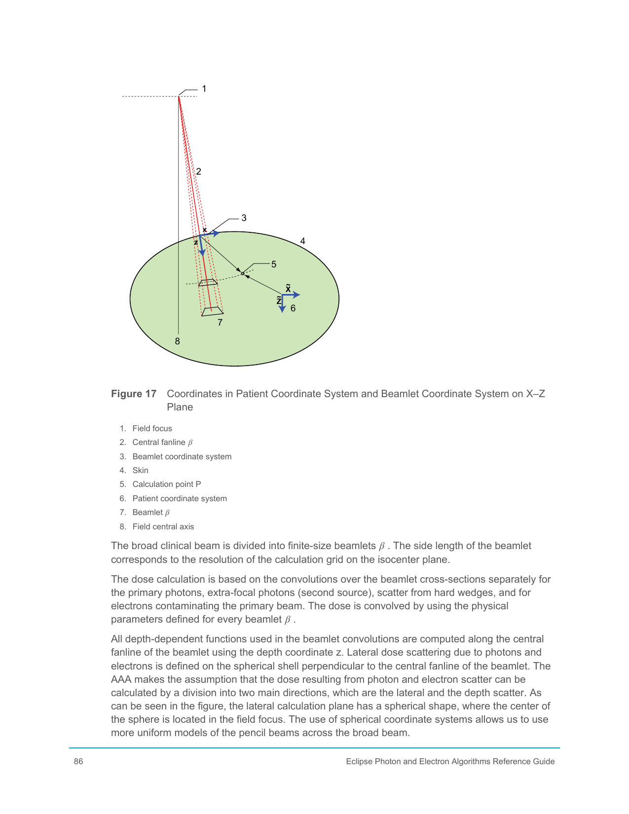
Each beamlet acts as a local calculation unit. Instead of treating the entire field as a single object, AAA sums the contributions of many small beam elements. That keeps the logic of the pencil beam family while making it much more powerful once it is combined with Monte Carlo-derived kernels and anisotropic heterogeneity scaling.

In the Varian manual, the lateral width of a beamlet is tied to the selected calculation resolution in the isocenter plane. That detail is clinically important. Grid resolution is not only a display choice. It also affects how the field is discretized internally.

Each beamlet carries:

• local fluence;
• spectral weighting;
• geometric position;
• the parameters required for longitudinal deposition and lateral scatter.

Dose at a given point is then obtained by superposing the contributions of all relevant beamlets. That architecture helps explain why AAA remained fast enough for routine planning while still handling fairly complex fields.

The central expression in AAA

The Varian manual presents the energy associated with a beamlet using an expression of the form:

This compact expression is one of the best ways to understand the algorithm because it condenses its core logic.

Fluence term: Φβ

This term represents how much radiation that beamlet carries. Source shaping, collimation, and beam modulation all influence it.

Longitudinal term: Iβ(z,ρ)

This term describes how energy is deposited along depth for that beamlet, taking tissue density into account. It captures attenuation and the depth-dependent behavior of the beam.

Lateral kernel: Kβ(X,Y,Z)

This kernel distributes energy laterally around the beamlet path. That is one of the pieces that makes AAA much more capable than simplified pencil beam models.

The key point is that AAA does not apply one global correction to the entire field. It combines a local fluence description, a local longitudinal deposition term, and a local lateral spread term for each beamlet.

Radiological depth: where heterogeneity really enters

One of the central ideas in AAA is the use of radiological depth rather than geometric depth alone:

This equation looks simple, but it carries an important physical interpretation. The algorithm attempts to rewrite a heterogeneous beam path as an equivalent water path, weighted by relative density.

That is exactly what allows AAA to improve substantially over older methods. The beam does not just “see” how many centimeters it has traveled. It sees how many radiological centimeters it has crossed.

But this is also where a conceptual limitation appears. Radiological depth handles part of the heterogeneity problem mainly along the main beam direction. It does not, by itself, resolve all the lateral transport effects associated with loss of charged-particle equilibrium or complex interface physics. That is why AAA improves strongly over classical pencil beam methods without becoming explicit transport.

The lateral kernel and what “anisotropic” really means

The word anisotropic in AAA is not decoration. It points to one of the algorithm’s most important upgrades.

Classical pencil beam approaches often assume a fairly simple lateral dose-spread behavior. AAA goes further by allowing the lateral energy redistribution to respond to the medium in a direction-dependent way. In the Varian documentation, the lateral kernel is represented through a sum of terms with depth-dependent coefficients:

You do not need to read this as a full derivation to understand its significance. The important point is that lateral spread is not treated as a fixed blur. It changes with radiological depth and with the beamlet context.

That is a major reason why AAA behaves much better than simple pencil beam engines near density changes and in fields where lateral scatter matters.

Why the algorithm is built around energy, not just dose

Another useful reading of AAA is that it is fundamentally an energy-transport approximation before it becomes a displayed dose map. The kernels are derived from Monte Carlo data and then scaled to clinical conditions. That matters because it anchors the algorithm in a physically informed representation of how secondary particles spread energy around the primary beam path.

This is also why AAA should not be dismissed as “old-fashioned” just because newer transport engines exist. Within its own family, it brought a real increase in physical realism.

Separate beam components matter clinically

The Varian documentation also emphasizes that AAA handles beam components separately:

• primary photons;
• extra-focal photons;
• wedge-related scatter;
• electron contamination.

That separation improves:

• surface dose behavior;
• penumbra description;
• near-edge dose;
• the handling of modified fields.

For example, electron contamination is modeled with its own depth dependence and lateral parameters. This is one reason why AAA behaves much better than simplified pencil beam models in shallow regions where surface and build-up behavior matter.

At the same time, this reminds us of something every physicist already knows but many comparisons ignore: a strong dose algorithm still depends on a strong beam model. If source settings, contamination parameters, or beam data are poor, the label AAA will not rescue the calculation.

Where AAA remains strong clinically

AAA is still a very competent algorithm across a large part of the photon-planning routine. Its strength comes from the combination of:

• a solid source model;
• anisotropic lateral-spread handling;
• Monte Carlo-derived kernels;
• calculation times compatible with optimization and routine planning.

It generally performs very well in:

• conventional 3D-CRT;
• a large share of IMRT and VMAT workflows;
• moderate heterogeneity scenarios;
• cases where the gain over classical pencil beam matters much more than the incremental gain from explicit transport.

This is the real reason AAA occupied such stable clinical ground for so long. It delivers a level of physical fidelity that is already decisive for many practical cases without imposing the heavier operational cost of transport solvers.

Where Varian itself recommends caution

The healthiest way to read a commercial algorithm is not to look only at what it does well. It is also to look carefully at what the manufacturer explicitly flags as a limitation.

In the Eclipse guide, Varian calls attention to known AAA limitations, especially in lung. There is a direct warning that when the beam crosses lung and then re-enters soft tissue, the algorithm tends to overestimate dose at the exit interface. The effect becomes more pronounced as the interface lies deeper in the beam path.

That statement deserves to be read slowly. It is not a random failure. It is a structural limitation tied to the kind of approximation the algorithm uses to represent transport and scatter in strongly heterogeneous media.

The manual also mentions performance differences in scenarios involving:

• specific field sizes and energies in lung;
• static MLC-defined fields under certain conditions;
• physical wedges;
• supports and high-density structures.

This is exactly the kind of guidance that should shape clinical judgment. An algorithm does not have to be rejected for its weaknesses to be taken seriously. What makes no sense is to use a scaled-kernel engine in a highly critical heterogeneity case and then act surprised when a more physical motor shifts the dose interpretation.

Grid resolution is not a side issue

The Eclipse guide also highlights something often treated as merely operational: grid resolution.

In AAA, the resolution typically ranges from 1 to 5 mm, and dose is first computed in a divergent matrix before being converted to the output grid. The relation between selected resolution, pixel spacing, and slice separation affects how the final dose is sampled.

That has real consequences. In high-gradient regions or in small fields, apparent algorithm behavior can change substantially with grid choice. In other words, part of what is sometimes reported as “difference between algorithms” is really a difference between discretizations of the same physical problem.

Methodologically, the implication is straightforward: comparing AAA with any serious transport engine without controlling for grid, slice spacing, and sampling parameters is not a clean comparison.

AAA is not a lighter Acuros

A recurring mistake is to think of AAA as if it were simply a lighter version of Acuros. It is not.

The two algorithms share part of the beam modeling, but they belong to different conceptual families:

Aspect	AAA	Acuros XB
Family	Beamlet-based convolution/superposition	Numerical solution of the LBTE
Main physical basis	Monte Carlo-derived kernels and radiological scaling	Explicit discretized transport in space, energy, and angle
Most central image quantity	Electron density	Mass density and material composition
Classical weakness	Strong heterogeneous interfaces, especially lung	Sensitivity to discretization and material mapping

That conceptual distinction matters because it changes both case interpretation and validation strategy.

When AAA is still the right choice

There is a current temptation to treat older engines as if they were automatically inferior in every setting. That is poor reading.

AAA still makes very good clinical sense when:

• the case is not dominated by extreme heterogeneity;
• the workflow needs speed without giving up solid physics;
• the institution knows its beam model well;
• comparison with more physical engines does not materially change the clinical decision.

That is why AAA remains relevant. It is not an outdated engine that happened to survive. It is a carefully built compromise between source modeling, Monte Carlo-derived kernels, clinical speed, and a far more serious treatment of heterogeneity than classical pencil beam ever offered.

That is also what explains its limits. In lung, at strong interfaces, and in scenarios where lateral transport dominates the problem, AAA still belongs to the world of scaled kernels. It can go very far inside that family, but it does not become explicit transport by approximation.

Reading the algorithm this way is more useful than repeating labels. It helps answer the practical questions that matter: when AAA is still the right engine, when recalculation with a more physical solver is worth the effort, and which discrepancies should be read as expected limitations rather than as a surprise from the TPS.